Simulating gamma-ray transport in the atmosphere using the spherical mass model
This tutorial will demonstrate the basic functionality of the spherical atmospheric mass model. For more details about the simulation and analysis pipeline, see Atmospheric Response for MeV Gamma Rays Observed with Balloon-Borne Detectors (Karwin+24).
Imports:
[1]:
from cosi_atmosphere.response.AtmosphericProfile import Atmosphere
from cosi_atmosphere.response.MassModels import MakeMassModels
from cosi_atmosphere.response.RunSims import Simulate
from cosi_atmosphere.response.ProcessSphericalSims import ProcessSpherical
import numpy as np
import os
This tutorial requires two files, which contain the photon data for a simulation using 1e7 photons. The files are hosted on wasabi, and they can be downloaded using the two cells below.
[ ]:
# File size: ~ 1GB
os.system("AWS_ACCESS_KEY_ID=GBAL6XATQZNRV3GFH9Y4 AWS_SECRET_ACCESS_KEY=GToOczY5hGX3sketNO2fUwiq4DJoewzIgvTCHoOv aws s3api get-object  --bucket cosi-pipeline-public --key COSI-Atmosphere/Spherical_Mass_Model_Tutorial/event_list_combined.dat --endpoint-url=https://s3.us-west-1.wasabisys.com event_list_combined.dat")
[ ]:
# File size: ~ 1.2GB
os.system("AWS_ACCESS_KEY_ID=GBAL6XATQZNRV3GFH9Y4 AWS_SECRET_ACCESS_KEY=GToOczY5hGX3sketNO2fUwiq4DJoewzIgvTCHoOv aws s3api get-object  --bucket cosi-pipeline-public --key COSI-Atmosphere/Spherical_Mass_Model_Tutorial/all_thrown_events_combined.dat --endpoint-url=https://s3.us-west-1.wasabisys.com all_thrown_events_combined.dat")
Make mass model
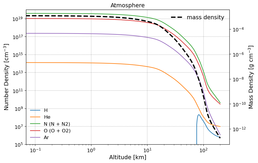
First, we need a model of the atmosphere. In general, this is dependent on location (latitude, longitude, altitude), time (year and day), and solar and geomagnetic activity levels. For our model we use a representative date, geographical location, and altitude from the COSI balloon flight.
[2]:
instance = Atmosphere()
date = np.array(['2016-06-13 12:00:00'], dtype="datetime64[h]")
lat = -5.66
lon = -107.38
alts = np.linspace(0, 200, 2001) # km; spacing is 0.1 km (100 m)
atm_model = instance.get_atm_profile("rep_atm_model.dat",date,lon,lat,alts)
The atmospheric model specifies the altitude profile of the number density for the primary species of the atmosphere (i.e. nitrogen, oxygen, argon, and helium). Let’s take a look at the first few lines of the output file:
[3]:
%%capture
os.system("head -n 5 rep_atm_model.dat")
altitude[km]    mass_density[kg/m3]     N2[m-3] O2[m-3] O[m-3]  He[m-3] H[m-3]  Ar[m-3] N[m-3]  anomalous_oxygen[m-3]   NO[m-3] Temperature[k]
0.000000e+00    1.176653e+00    1.911429e+25    5.125639e+24    0.000000e+00    1.272904e+20    0.000000e+00    2.284374e+23    0.000000e+00    0.000000e+00    0.000000e+00    2.966827e+02
1.000000e-01    1.164742e+00    1.892081e+25    5.073756e+24    0.000000e+00    1.260020e+20    0.000000e+00    2.261251e+23    0.000000e+00    0.000000e+00    0.000000e+00    2.962918e+02
2.000000e-01    1.152961e+00    1.872944e+25    5.022437e+24    0.000000e+00    1.247275e+20    0.000000e+00    2.238379e+23    0.000000e+00    0.000000e+00    0.000000e+00    2.958947e+02
3.000000e-01    1.141304e+00    1.854006e+25    4.971656e+24    0.000000e+00    1.234664e+20    0.000000e+00    2.215747e+23    0.000000e+00    0.000000e+00    0.000000e+00    2.954918e+02
Now we can make our mass model. Let’s first take a look at the atmospheric profiles:
[4]:
instance = MakeMassModels("rep_atm_model.dat")
instance.plot_atmosphere()
We’ll use the spherical mass model, which consists of spherical shells with a thickness of 100 meters (as defined in the atmospheric profile). In order to track photons, we’ll place our watched volume (consisting of a spherical shell) at an altitude of 33.5 km. We can use different altitudes if we want. Note that the spherical shells are defined relative to Earth’s radius.
[5]:
instance.spherical_model(33.5)
Using shell thickness [cm]: 10000.0
Watch index: 335
The mass model is written to a standard MEGAlib geo file. Let’s take a look at the first 50 lines:
[6]:
%%capture
os.system("head -n 50 atmosphere.geo")
# Atmosphere model

Name AtmoshpereModel

# Surrounding sphere:
SurroundingSphere 657800000.0 0 0 0 657800000.0
ShowSurroundingSphere true

Volume World
World.Material Vacuum
World.Shape BOX 10240000000.000000 10240000000.000000 10240000000.000000
World.Visibility 1
World.Position 0 0 0
World.Mother 0

Include $(MEGALIB)/resource/examples/geomega/materials/Materials.geo

Material MaterialSlice_0_1
MaterialSlice_0_1.Density 0.001176653
MaterialSlice_0_1.ComponentByAtoms He 2
MaterialSlice_0_1.ComponentByAtoms N 784845
MaterialSlice_0_1.ComponentByAtoms O 210462
MaterialSlice_0_1.ComponentByAtoms Ar 4689

Volume VolumeSlice_0_1
VolumeSlice_0_1.Material MaterialSlice_0_1
VolumeSlice_0_1.Shape SPHERE 637800000.0 637810000.0
VolumeSlice_0_1.Visibility  0
VolumeSlice_0_1.Position 0 0 0
VolumeSlice_0_1.Color 7
VolumeSlice_0_1.Mother World

Material MaterialSlice_1_2
MaterialSlice_1_2.Density 0.0011647419999999999
MaterialSlice_1_2.ComponentByAtoms He 2
MaterialSlice_1_2.ComponentByAtoms N 784845
MaterialSlice_1_2.ComponentByAtoms O 210462
MaterialSlice_1_2.ComponentByAtoms Ar 4689

Volume VolumeSlice_1_2
VolumeSlice_1_2.Material MaterialSlice_1_2
VolumeSlice_1_2.Shape SPHERE 637810000.0 637820000.0
VolumeSlice_1_2.Visibility  0
VolumeSlice_1_2.Position 0 0 0
VolumeSlice_1_2.Color 0
VolumeSlice_1_2.Mother World

Material MaterialSlice_2_3
MaterialSlice_2_3.Density 0.0011529609999999999
MaterialSlice_2_3.ComponentByAtoms He 2
The watched volume is specified at the end of the file. Let’s take a look:
[7]:
%%capture
os.system("tail -n 8 atmosphere.geo")
Volume TestSphere
TestSphere.Material MaterialSlice_335_336
TestSphere.Shape Sphere 641150000.0 641160000.0
TestSphere.Visibility 1
TestSphere.Position 0 0 0
TestSphere.Color 2
TestSphere.Mother VolumeSlice_335_336
Run Simulations
Now we can run the simulations. We simulate an isotropic source with a flat energy spectrum (i.e. constant number of photons per energy bin) between 10 keV - 10 MeV. The source is simulated using a surrounding sphere with a radius of 200 km. The simulations should use at least 1e7 photons, but here we’ll just simulate 100, just as a simple demonstration.
[8]:
instance = Simulate()
instance.run_sim("Atmosphere_Isotropic.source")
**************************************************************************
*                                                                        *
*                Cosima - the cosmic simulator of MEGAlib                *
*                                                                        *
*             This program is part of MEGAlib version 3.99.02            *
*                (C) by Andreas Zoglauer and contributors                *
*                                                                        *
*                      Master reference for MEGAlib:                     *
*            A. Zoglauer et al., NewAR 50 (7-8), 629-632, 2006           *
*                                                                        *
*            For more information about MEGAlib please visit:            *
*                        http://megalibtoolkit.com                       *
*                                                                        *
**************************************************************************

              You are using a development version of MEGAlib

Using verbosity 1
Using parameter file Atmosphere_Isotropic.source
Deprecated: Fluorescence is activated by default where possible.
Info: StoreOnlyTriggeredEvents is deprecated. Please use PreTriggerMode

*************************************************************
 Geant4 version Name: geant4-10-02-patch-03    (27-January-2017)
                      Copyright : Geant4 Collaboration
                      Reference : NIM A 506 (2003), 250-303
                            WWW : http://cern.ch/geant4
*************************************************************

Chosen physics:
Particles
G4EmLivermorePolarizedPhysics
G4RadioactiveDecay

Stage 1 (reading of file(s)) finished after 0.107719 sec
Stage 2 (evaluating constants and maths) finished after 0.159505 sec
Stage 3 (evaluating vectors) finished after 0.1731 sec
Stage 4 (evaluating for loops) finished after 0.185967 sec
Stage 5 (evaluating random numbers) finished after 0.189584 sec
Stage 6 (evaluating if clauses + initial maths evaluation) finished after 0.241681 sec
Stage 7 (analyzing primary keywords) finished after 0.664411 sec
Stage 8 (analyzing "Copies") finished after 0.676833 sec
Stage 9 (analyzing all properties) finished after 7.27866 sec
Stage 10 (generating clones) finished after 7.27987 sec
   ***  Warning  ***
You have not defined any trigger criteria!!
Stage 11 (validation & post-processing) finished after 7.78577 sec
Stage 12 (volume tree optimization) finished after 7.78593 sec
Beam: average start area: 1.35937e+18 cm2
Beam: Final flux: 1 ph/cm^2/sec
Visualization Manager instantiating with verbosity "warnings (3)"...
Visualization Manager initialising...
Registering graphics systems...

You have successfully registered the following graphics systems.
Current available graphics systems are:
ASCIITree (ATree)
DAWNFILE (DAWNFILE)
G4HepRep (HepRepXML)
G4HepRepFile (HepRepFile)
RayTracer (RayTracer)
VRML1FILE (VRML1FILE)
VRML2FILE (VRML2FILE)
gMocrenFile (gMocrenFile)

Registering model factories...

You have successfully registered the following model factories.
Registered model factories:
  generic
  drawByCharge
  drawByParticleID
  drawByOriginVolume
  drawByAttribute

Registered filter factories:
  chargeFilter
  particleFilter
  originVolumeFilter
  attributeFilter

You have successfully registered the following user vis actions.
Run Duration User Vis Actions: none
End of Event User Vis Actions: none
End of Run User Vis Actions: none

Some /vis commands (optionally) take a string to specify colour.
Available colours:
  black, blue, brown, cyan, gray, green, grey, magenta, red, white, yellow


Starting run "SpaceSim":


### ===  Deexcitation model UAtomDeexcitation is activated for 1 region:
          DefaultRegionForTheWorld

### === G4UAtomicDeexcitation::InitialiseForNewRun()
### ===  PIXE model for hadrons: Empirical
### ===  PIXE model for e+-:     Livermore

phot:   for  gamma    SubType= 12  BuildTable= 0
      LambdaPrime table from 200 keV to 10 TeV in 154 bins
      ===== EM models for the G4Region  DefaultRegionForTheWorld ======
LivermorePolarizedPhotoElectric :  Emin=        0 eV    Emax=        1 GeV   AngularGenSauterGavrilaPolarized  FluoActive
       PhotoElectric :  Emin=        1 GeV   Emax=       10 TeV   AngularGenSauterGavrila  FluoActive

compt:   for  gamma    SubType= 13  BuildTable= 1
      Lambda table from 100 eV  to 1 MeV, 20 bins per decade, spline: 1
      LambdaPrime table from 1 MeV to 10 TeV in 140 bins
      ===== EM models for the G4Region  DefaultRegionForTheWorld ======
LivermorePolarizedCompton :  Emin=        0 eV    Emax=        1 GeV  FluoActive
       Klein-Nishina :  Emin=        1 GeV   Emax=       10 TeV

conv:   for  gamma    SubType= 14  BuildTable= 1
      Lambda table from 1.022 MeV to 10 TeV, 20 bins per decade, spline: 1
      ===== EM models for the G4Region  DefaultRegionForTheWorld ======
LivermorePolarizedGammaConversion :  Emin=        0 eV    Emax=        1 GeV
        BetheHeitler :  Emin=        1 GeV   Emax=       80 GeV
     BetheHeitlerLPM :  Emin=       80 GeV   Emax=       10 TeV

Rayl:   for  gamma    SubType= 11  BuildTable= 1
      Lambda table from 100 eV  to 100 keV, 20 bins per decade, spline: 0
      LambdaPrime table from 100 keV to 10 TeV in 160 bins
      ===== EM models for the G4Region  DefaultRegionForTheWorld ======
LivermorePolarizedRayleigh :  Emin=        0 eV    Emax=        1 GeV
   LivermoreRayleigh :  Emin=        1 GeV   Emax=       10 TeV   CullenGenerator

msc:   for e-    SubType= 10
      RangeFactor= 0.04, stepLimitType: 3, latDisplacement: 1, skin= 1, geomFactor= 2.5
      ===== EM models for the G4Region  DefaultRegionForTheWorld ======
            UrbanMsc :  Emin=        0 eV    Emax=      100 MeV  Table with 120 bins Emin=    100 eV    Emax=    100 MeV
        WentzelVIUni :  Emin=      100 MeV   Emax=       10 TeV  Table with 100 bins Emin=    100 MeV   Emax=     10 TeV

CoulombScat:   for  e-, integral: 1     SubType= 1  BuildTable= 1
      Lambda table from 100 MeV to 10 TeV, 20 bins per decade, spline: 1
      180 < Theta(degree) < 180; pLimit(GeV^1)= 0.139531
      ===== EM models for the G4Region  DefaultRegionForTheWorld ======
  eCoulombScattering :  Emin=      100 MeV   Emax=       10 TeV

eIoni:   for  e-    SubType= 2
      dE/dx and range tables from 100 eV  to 10 TeV in 220 bins
      Lambda tables from threshold to 10 TeV, 20 bins per decade, spline: 1
      finalRange(mm)= 0.1, dRoverRange= 0.2, integral: 1, fluct: 1, linLossLimit= 0.01
      ===== EM models for the G4Region  DefaultRegionForTheWorld ======
       LowEnergyIoni :  Emin=        0 eV    Emax=      100 keV   deltaVI
        MollerBhabha :  Emin=      100 keV   Emax=       10 TeV   deltaVI

eBrem:   for  e-    SubType= 3
      dE/dx and range tables from 100 eV  to 10 TeV in 220 bins
      Lambda tables from threshold to 10 TeV, 20 bins per decade, spline: 1
      LPM flag: 1 for E > 1 GeV,  HighEnergyThreshold(GeV)= 10000
      ===== EM models for the G4Region  DefaultRegionForTheWorld ======
             eBremSB :  Emin=        0 eV    Emax=        1 GeV   DipBustGen
            eBremLPM :  Emin=        1 GeV   Emax=       10 TeV   DipBustGen

msc:   for e+    SubType= 10
      RangeFactor= 0.04, stepLimitType: 3, latDisplacement: 1, skin= 1, geomFactor= 2.5
      ===== EM models for the G4Region  DefaultRegionForTheWorld ======
            UrbanMsc :  Emin=        0 eV    Emax=      100 MeV  Table with 120 bins Emin=    100 eV    Emax=    100 MeV
        WentzelVIUni :  Emin=      100 MeV   Emax=       10 TeV  Table with 100 bins Emin=    100 MeV   Emax=     10 TeV

eIoni:   for  e+    SubType= 2
      dE/dx and range tables from 100 eV  to 10 TeV in 220 bins
      Lambda tables from threshold to 10 TeV, 20 bins per decade, spline: 1
      finalRange(mm)= 0.1, dRoverRange= 0.2, integral: 1, fluct: 1, linLossLimit= 0.01
      ===== EM models for the G4Region  DefaultRegionForTheWorld ======
        MollerBhabha :  Emin=        0 eV    Emax=       10 TeV   deltaVI

eBrem:   for  e+    SubType= 3
      dE/dx and range tables from 100 eV  to 10 TeV in 220 bins
      Lambda tables from threshold to 10 TeV, 20 bins per decade, spline: 1
      LPM flag: 1 for E > 1 GeV,  HighEnergyThreshold(GeV)= 10000
      ===== EM models for the G4Region  DefaultRegionForTheWorld ======
             eBremSB :  Emin=        0 eV    Emax=        1 GeV   DipBustGen
            eBremLPM :  Emin=        1 GeV   Emax=       10 TeV   DipBustGen

annihil:   for  e+, integral: 1     SubType= 5  BuildTable= 0
      ===== EM models for the G4Region  DefaultRegionForTheWorld ======
            eplus2gg :  Emin=        0 eV    Emax=       10 TeV

CoulombScat:   for  e+, integral: 1     SubType= 1  BuildTable= 1
      Lambda table from 100 MeV to 10 TeV, 20 bins per decade, spline: 1
      180 < Theta(degree) < 180; pLimit(GeV^1)= 0.139531
      ===== EM models for the G4Region  DefaultRegionForTheWorld ======
  eCoulombScattering :  Emin=      100 MeV   Emax=       10 TeV

msc:   for proton    SubType= 10
      RangeFactor= 0.2, step limit type: 0, lateralDisplacement: 0, polarAngleLimit(deg)= 180
      ===== EM models for the G4Region  DefaultRegionForTheWorld ======
        WentzelVIUni :  Emin=        0 eV    Emax=       10 TeV  Table with 220 bins Emin=    100 eV    Emax=     10 TeV

hIoni:   for  proton    SubType= 2
      dE/dx and range tables from 100 eV  to 10 TeV in 220 bins
      Lambda tables from threshold to 10 TeV, 20 bins per decade, spline: 1
      finalRange(mm)= 0.05, dRoverRange= 0.2, integral: 1, fluct: 1, linLossLimit= 0.01
      ===== EM models for the G4Region  DefaultRegionForTheWorld ======
               Bragg :  Emin=        0 eV    Emax=        2 MeV   deltaVI
          BetheBloch :  Emin=        2 MeV   Emax=       10 TeV   deltaVI

hBrems:   for  proton    SubType= 3
      dE/dx and range tables from 100 eV  to 10 TeV in 220 bins
      Lambda tables from threshold to 10 TeV, 20 bins per decade, spline: 1
      ===== EM models for the G4Region  DefaultRegionForTheWorld ======
               hBrem :  Emin=        0 eV    Emax=       10 TeV

hPairProd:   for  proton    SubType= 4
      dE/dx and range tables from 100 eV  to 10 TeV in 220 bins
      Lambda tables from threshold to 10 TeV, 20 bins per decade, spline: 1
      Sampling table 13x1001; from 7.50618 GeV to 10 TeV
      ===== EM models for the G4Region  DefaultRegionForTheWorld ======
           hPairProd :  Emin=        0 eV    Emax=       10 TeV

nuclearStopping:   for  proton    SubType= 8  BuildTable= 0
      ===== EM models for the G4Region  DefaultRegionForTheWorld ======
   ICRU49NucStopping :  Emin=        0 eV    Emax=        1 MeV

CoulombScat:   for  proton, integral: 1     SubType= 1  BuildTable= 1
      Lambda table from threshold  to 10 TeV, 20 bins per decade, spline: 1
      180 < Theta(degree) < 180; pLimit(GeV^1)= 0.139531
      ===== EM models for the G4Region  DefaultRegionForTheWorld ======
  eCoulombScattering :  Emin=        0 eV    Emax=       10 TeV

msc:   for GenericIon    SubType= 10
      RangeFactor= 0.2, stepLimitType: 0, latDisplacement: 0
      ===== EM models for the G4Region  DefaultRegionForTheWorld ======
            UrbanMsc :  Emin=        0 eV    Emax=       10 TeV

ionIoni:   for  GenericIon    SubType= 2
      dE/dx and range tables from 100 eV  to 10 TeV in 220 bins
      Lambda tables from threshold to 10 TeV, 20 bins per decade, spline: 1
      finalRange(mm)= 0.001, dRoverRange= 0.1, integral: 1, fluct: 1, linLossLimit= 0.02
      ===== EM models for the G4Region  DefaultRegionForTheWorld ======
         ParamICRU73 :  Emin=        0 eV    Emax=       10 TeV   deltaVI

nuclearStopping:   for  GenericIon    SubType= 8  BuildTable= 0
      ===== EM models for the G4Region  DefaultRegionForTheWorld ======
   ICRU49NucStopping :  Emin=        0 eV    Emax=        1 MeV

### ===  Deexcitation model UAtomDeexcitation is activated for 1 region:
          DefaultRegionForTheWorld

### === G4UAtomicDeexcitation::InitialiseForNewRun()
### ===  PIXE model for hadrons: Empirical
### ===  PIXE model for e+-:     Livermore

msc:   for alpha    SubType= 10
      RangeFactor= 0.2, stepLimitType: 0, latDisplacement: 0
      ===== EM models for the G4Region  DefaultRegionForTheWorld ======
            UrbanMsc :  Emin=        0 eV    Emax=       10 TeV  Table with 220 bins Emin=    100 eV    Emax=     10 TeV

ionIoni:   for  alpha    SubType= 2
      dE/dx and range tables from 100 eV  to 10 TeV in 220 bins
      Lambda tables from threshold to 10 TeV, 20 bins per decade, spline: 1
      finalRange(mm)= 0.01, dRoverRange= 0.1, integral: 1, fluct: 1, linLossLimit= 0.02
      ===== EM models for the G4Region  DefaultRegionForTheWorld ======
            BraggIon :  Emin=        0 eV    Emax=   7.9452 MeV   deltaVI
          BetheBloch :  Emin=   7.9452 MeV   Emax=       10 TeV   deltaVI

nuclearStopping:   for  alpha    SubType= 8  BuildTable= 0
      ===== EM models for the G4Region  DefaultRegionForTheWorld ======
   ICRU49NucStopping :  Emin=        0 eV    Emax=        1 MeV

msc:   for anti_proton    SubType= 10
      RangeFactor= 0.2, step limit type: 0, lateralDisplacement: 0, polarAngleLimit(deg)= 180
      ===== EM models for the G4Region  DefaultRegionForTheWorld ======
        WentzelVIUni :  Emin=        0 eV    Emax=       10 TeV  Table with 220 bins Emin=    100 eV    Emax=     10 TeV

hIoni:   for  anti_proton    SubType= 2
      dE/dx and range tables from 100 eV  to 10 TeV in 220 bins
      Lambda tables from threshold to 10 TeV, 20 bins per decade, spline: 1
      finalRange(mm)= 0.05, dRoverRange= 0.2, integral: 1, fluct: 1, linLossLimit= 0.01
      ===== EM models for the G4Region  DefaultRegionForTheWorld ======
            ICRU73QO :  Emin=        0 eV    Emax=        2 MeV   deltaVI
          BetheBloch :  Emin=        2 MeV   Emax=       10 TeV   deltaVI

hBrems:   for  anti_proton    SubType= 3
      dE/dx and range tables from 100 eV  to 10 TeV in 220 bins
      Lambda tables from threshold to 10 TeV, 20 bins per decade, spline: 1
      ===== EM models for the G4Region  DefaultRegionForTheWorld ======
               hBrem :  Emin=        0 eV    Emax=       10 TeV

hPairProd:   for  anti_proton    SubType= 4
      dE/dx and range tables from 100 eV  to 10 TeV in 220 bins
      Lambda tables from threshold to 10 TeV, 20 bins per decade, spline: 1
      Sampling table 13x1001; from 7.50618 GeV to 10 TeV
      ===== EM models for the G4Region  DefaultRegionForTheWorld ======
           hPairProd :  Emin=        0 eV    Emax=       10 TeV

nuclearStopping:   for  anti_proton    SubType= 8  BuildTable= 0
      ===== EM models for the G4Region  DefaultRegionForTheWorld ======
   ICRU49NucStopping :  Emin=        0 eV    Emax=        1 MeV

CoulombScat:   for  anti_proton, integral: 1     SubType= 1  BuildTable= 1
      Lambda table from threshold  to 10 TeV, 20 bins per decade, spline: 1
      180 < Theta(degree) < 180; pLimit(GeV^1)= 0.139531
      ===== EM models for the G4Region  DefaultRegionForTheWorld ======
  eCoulombScattering :  Emin=        0 eV    Emax=       10 TeV

msc:   for kaon+    SubType= 10
      RangeFactor= 0.2, step limit type: 0, lateralDisplacement: 0, polarAngleLimit(deg)= 180
      ===== EM models for the G4Region  DefaultRegionForTheWorld ======
        WentzelVIUni :  Emin=        0 eV    Emax=       10 TeV  Table with 220 bins Emin=    100 eV    Emax=     10 TeV

hIoni:   for  kaon+    SubType= 2
      dE/dx and range tables from 100 eV  to 10 TeV in 220 bins
      Lambda tables from threshold to 10 TeV, 20 bins per decade, spline: 1
      finalRange(mm)= 0.05, dRoverRange= 0.2, integral: 1, fluct: 1, linLossLimit= 0.01
      ===== EM models for the G4Region  DefaultRegionForTheWorld ======
               Bragg :  Emin=        0 eV    Emax=  1.05231 MeV   deltaVI
          BetheBloch :  Emin=  1.05231 MeV   Emax=       10 TeV   deltaVI

hBrems:   for  kaon+    SubType= 3
      dE/dx and range tables from 100 eV  to 10 TeV in 220 bins
      Lambda tables from threshold to 10 TeV, 20 bins per decade, spline: 1
      ===== EM models for the G4Region  DefaultRegionForTheWorld ======
               hBrem :  Emin=        0 eV    Emax=       10 TeV

hPairProd:   for  kaon+    SubType= 4
      dE/dx and range tables from 100 eV  to 10 TeV in 220 bins
      Lambda tables from threshold to 10 TeV, 20 bins per decade, spline: 1
      Sampling table 14x1001; from 3.94942 GeV to 10 TeV
      ===== EM models for the G4Region  DefaultRegionForTheWorld ======
           hPairProd :  Emin=        0 eV    Emax=       10 TeV

CoulombScat:   for  kaon+, integral: 1     SubType= 1  BuildTable= 1
      Lambda table from threshold  to 10 TeV, 20 bins per decade, spline: 1
      180 < Theta(degree) < 180; pLimit(GeV^1)= 0.139531
      ===== EM models for the G4Region  DefaultRegionForTheWorld ======
  eCoulombScattering :  Emin=        0 eV    Emax=       10 TeV

msc:   for kaon-    SubType= 10
      RangeFactor= 0.2, step limit type: 0, lateralDisplacement: 0, polarAngleLimit(deg)= 180
      ===== EM models for the G4Region  DefaultRegionForTheWorld ======
        WentzelVIUni :  Emin=        0 eV    Emax=       10 TeV  Table with 220 bins Emin=    100 eV    Emax=     10 TeV

hIoni:   for  kaon-    SubType= 2
      dE/dx and range tables from 100 eV  to 10 TeV in 220 bins
      Lambda tables from threshold to 10 TeV, 20 bins per decade, spline: 1
      finalRange(mm)= 0.05, dRoverRange= 0.2, integral: 1, fluct: 1, linLossLimit= 0.01
      ===== EM models for the G4Region  DefaultRegionForTheWorld ======
            ICRU73QO :  Emin=        0 eV    Emax=  1.05231 MeV   deltaVI
          BetheBloch :  Emin=  1.05231 MeV   Emax=       10 TeV   deltaVI

hBrems:   for  kaon-    SubType= 3
      dE/dx and range tables from 100 eV  to 10 TeV in 220 bins
      Lambda tables from threshold to 10 TeV, 20 bins per decade, spline: 1
      ===== EM models for the G4Region  DefaultRegionForTheWorld ======
               hBrem :  Emin=        0 eV    Emax=       10 TeV

hPairProd:   for  kaon-    SubType= 4
      dE/dx and range tables from 100 eV  to 10 TeV in 220 bins
      Lambda tables from threshold to 10 TeV, 20 bins per decade, spline: 1
      Sampling table 14x1001; from 3.94942 GeV to 10 TeV
      ===== EM models for the G4Region  DefaultRegionForTheWorld ======
           hPairProd :  Emin=        0 eV    Emax=       10 TeV

CoulombScat:   for  kaon-, integral: 1     SubType= 1  BuildTable= 1
      Lambda table from threshold  to 10 TeV, 20 bins per decade, spline: 1
      180 < Theta(degree) < 180; pLimit(GeV^1)= 0.139531
      ===== EM models for the G4Region  DefaultRegionForTheWorld ======
  eCoulombScattering :  Emin=        0 eV    Emax=       10 TeV

msc:   for mu+    SubType= 10
      RangeFactor= 0.2, step limit type: 0, lateralDisplacement: 0, polarAngleLimit(deg)= 180
      ===== EM models for the G4Region  DefaultRegionForTheWorld ======
        WentzelVIUni :  Emin=        0 eV    Emax=       10 TeV  Table with 220 bins Emin=    100 eV    Emax=     10 TeV

muIoni:   for  mu+    SubType= 2
      dE/dx and range tables from 100 eV  to 10 TeV in 220 bins
      Lambda tables from threshold to 10 TeV, 20 bins per decade, spline: 1
      finalRange(mm)= 0.05, dRoverRange= 0.2, integral: 1, fluct: 1, linLossLimit= 0.01
      ===== EM models for the G4Region  DefaultRegionForTheWorld ======
               Bragg :  Emin=        0 eV    Emax=      200 keV   deltaVI
          BetheBloch :  Emin=      200 keV   Emax=        1 GeV   deltaVI
        MuBetheBloch :  Emin=        1 GeV   Emax=       10 TeV

muBrems:   for  mu+    SubType= 3
      dE/dx and range tables from 100 eV  to 10 TeV in 220 bins
      Lambda tables from threshold to 10 TeV, 20 bins per decade, spline: 1
      ===== EM models for the G4Region  DefaultRegionForTheWorld ======
              MuBrem :  Emin=        0 eV    Emax=       10 TeV

muPairProd:   for  mu+    SubType= 4
      dE/dx and range tables from 100 eV  to 10 TeV in 220 bins
      Lambda tables from threshold to 10 TeV, 20 bins per decade, spline: 1
      Sampling table 17x1001; from 1 GeV to 10 TeV
      ===== EM models for the G4Region  DefaultRegionForTheWorld ======
          muPairProd :  Emin=        0 eV    Emax=       10 TeV

CoulombScat:   for  mu+, integral: 1     SubType= 1  BuildTable= 1
      Lambda table from threshold  to 10 TeV, 20 bins per decade, spline: 1
      180 < Theta(degree) < 180; pLimit(GeV^1)= 0.139531
      ===== EM models for the G4Region  DefaultRegionForTheWorld ======
  eCoulombScattering :  Emin=        0 eV    Emax=       10 TeV

msc:   for mu-    SubType= 10
      RangeFactor= 0.2, step limit type: 0, lateralDisplacement: 0, polarAngleLimit(deg)= 180
      ===== EM models for the G4Region  DefaultRegionForTheWorld ======
        WentzelVIUni :  Emin=        0 eV    Emax=       10 TeV  Table with 220 bins Emin=    100 eV    Emax=     10 TeV

muIoni:   for  mu-    SubType= 2
      dE/dx and range tables from 100 eV  to 10 TeV in 220 bins
      Lambda tables from threshold to 10 TeV, 20 bins per decade, spline: 1
      finalRange(mm)= 0.05, dRoverRange= 0.2, integral: 1, fluct: 1, linLossLimit= 0.01
      ===== EM models for the G4Region  DefaultRegionForTheWorld ======
            ICRU73QO :  Emin=        0 eV    Emax=      200 keV   deltaVI
          BetheBloch :  Emin=      200 keV   Emax=        1 GeV   deltaVI
        MuBetheBloch :  Emin=        1 GeV   Emax=       10 TeV

muBrems:   for  mu-    SubType= 3
      dE/dx and range tables from 100 eV  to 10 TeV in 220 bins
      Lambda tables from threshold to 10 TeV, 20 bins per decade, spline: 1
      ===== EM models for the G4Region  DefaultRegionForTheWorld ======
              MuBrem :  Emin=        0 eV    Emax=       10 TeV

muPairProd:   for  mu-    SubType= 4
      dE/dx and range tables from 100 eV  to 10 TeV in 220 bins
      Lambda tables from threshold to 10 TeV, 20 bins per decade, spline: 1
      Sampling table 17x1001; from 1 GeV to 10 TeV
      ===== EM models for the G4Region  DefaultRegionForTheWorld ======
          muPairProd :  Emin=        0 eV    Emax=       10 TeV

CoulombScat:   for  mu-, integral: 1     SubType= 1  BuildTable= 1
      Lambda table from threshold  to 10 TeV, 20 bins per decade, spline: 1
      180 < Theta(degree) < 180; pLimit(GeV^1)= 0.139531
      ===== EM models for the G4Region  DefaultRegionForTheWorld ======
  eCoulombScattering :  Emin=        0 eV    Emax=       10 TeV

msc:   for pi+    SubType= 10
      RangeFactor= 0.2, step limit type: 0, lateralDisplacement: 0, polarAngleLimit(deg)= 180
      ===== EM models for the G4Region  DefaultRegionForTheWorld ======
        WentzelVIUni :  Emin=        0 eV    Emax=       10 TeV  Table with 220 bins Emin=    100 eV    Emax=     10 TeV

hIoni:   for  pi+    SubType= 2
      dE/dx and range tables from 100 eV  to 10 TeV in 220 bins
      Lambda tables from threshold to 10 TeV, 20 bins per decade, spline: 1
      finalRange(mm)= 0.05, dRoverRange= 0.2, integral: 1, fluct: 1, linLossLimit= 0.01
      ===== EM models for the G4Region  DefaultRegionForTheWorld ======
               Bragg :  Emin=        0 eV    Emax=  297.505 keV   deltaVI
          BetheBloch :  Emin=  297.505 keV   Emax=       10 TeV   deltaVI

hBrems:   for  pi+    SubType= 3
      dE/dx and range tables from 100 eV  to 10 TeV in 220 bins
      Lambda tables from threshold to 10 TeV, 20 bins per decade, spline: 1
      ===== EM models for the G4Region  DefaultRegionForTheWorld ======
               hBrem :  Emin=        0 eV    Emax=       10 TeV

hPairProd:   for  pi+    SubType= 4
      dE/dx and range tables from 100 eV  to 10 TeV in 220 bins
      Lambda tables from threshold to 10 TeV, 20 bins per decade, spline: 1
      Sampling table 16x1001; from 1.11656 GeV to 10 TeV
      ===== EM models for the G4Region  DefaultRegionForTheWorld ======
           hPairProd :  Emin=        0 eV    Emax=       10 TeV

CoulombScat:   for  pi+, integral: 1     SubType= 1  BuildTable= 1
      Lambda table from threshold  to 10 TeV, 20 bins per decade, spline: 1
      180 < Theta(degree) < 180; pLimit(GeV^1)= 0.139531
      ===== EM models for the G4Region  DefaultRegionForTheWorld ======
  eCoulombScattering :  Emin=        0 eV    Emax=       10 TeV

msc:   for pi-    SubType= 10
      RangeFactor= 0.2, step limit type: 0, lateralDisplacement: 0, polarAngleLimit(deg)= 180
      ===== EM models for the G4Region  DefaultRegionForTheWorld ======
        WentzelVIUni :  Emin=        0 eV    Emax=       10 TeV  Table with 220 bins Emin=    100 eV    Emax=     10 TeV

hIoni:   for  pi-    SubType= 2
      dE/dx and range tables from 100 eV  to 10 TeV in 220 bins
      Lambda tables from threshold to 10 TeV, 20 bins per decade, spline: 1
      finalRange(mm)= 0.05, dRoverRange= 0.2, integral: 1, fluct: 1, linLossLimit= 0.01
      ===== EM models for the G4Region  DefaultRegionForTheWorld ======
            ICRU73QO :  Emin=        0 eV    Emax=  297.505 keV   deltaVI
          BetheBloch :  Emin=  297.505 keV   Emax=       10 TeV   deltaVI

hBrems:   for  pi-    SubType= 3
      dE/dx and range tables from 100 eV  to 10 TeV in 220 bins
      Lambda tables from threshold to 10 TeV, 20 bins per decade, spline: 1
      ===== EM models for the G4Region  DefaultRegionForTheWorld ======
               hBrem :  Emin=        0 eV    Emax=       10 TeV

hPairProd:   for  pi-    SubType= 4
      dE/dx and range tables from 100 eV  to 10 TeV in 220 bins
      Lambda tables from threshold to 10 TeV, 20 bins per decade, spline: 1
      Sampling table 16x1001; from 1.11656 GeV to 10 TeV
      ===== EM models for the G4Region  DefaultRegionForTheWorld ======
           hPairProd :  Emin=        0 eV    Emax=       10 TeV

CoulombScat:   for  pi-, integral: 1     SubType= 1  BuildTable= 1
      Lambda table from threshold  to 10 TeV, 20 bins per decade, spline: 1
      180 < Theta(degree) < 180; pLimit(GeV^1)= 0.139531
      ===== EM models for the G4Region  DefaultRegionForTheWorld ======
  eCoulombScattering :  Emin=        0 eV    Emax=       10 TeV
Storing event 1 of 1 at t_obs=5.06165e-19s
Storing event 2 of 2 at t_obs=1.27465e-18s
Storing event 3 of 3 at t_obs=1.76096e-18s
Storing event 4 of 4 at t_obs=1.84561e-18s
Storing event 5 of 5 at t_obs=2.03024e-18s
Storing event 6 of 6 at t_obs=2.25077e-18s
Storing event 7 of 7 at t_obs=2.43874e-18s
Storing event 8 of 8 at t_obs=2.46908e-18s
Storing event 9 of 9 at t_obs=2.54623e-18s
Storing event 10 of 10 at t_obs=2.62152e-18s
Storing event 11 of 11 at t_obs=2.92185e-18s
Storing event 12 of 12 at t_obs=3.92299e-18s
Storing event 13 of 13 at t_obs=5.13114e-18s
Storing event 14 of 14 at t_obs=5.62943e-18s
Storing event 15 of 15 at t_obs=6.16729e-18s
Storing event 16 of 16 at t_obs=6.32382e-18s
Storing event 17 of 17 at t_obs=6.65867e-18s
Storing event 18 of 18 at t_obs=7.41556e-18s
Storing event 19 of 19 at t_obs=7.51617e-18s
Storing event 20 of 20 at t_obs=7.6204e-18s
Storing event 21 of 21 at t_obs=7.77669e-18s
Storing event 22 of 22 at t_obs=8.90907e-18s
Storing event 23 of 23 at t_obs=9.0672e-18s
Storing event 24 of 24 at t_obs=1.05062e-17s
Storing event 25 of 25 at t_obs=1.07009e-17s
Storing event 26 of 26 at t_obs=1.12727e-17s
Storing event 27 of 27 at t_obs=1.25958e-17s
Storing event 28 of 28 at t_obs=1.4018e-17s
Storing event 29 of 29 at t_obs=1.53312e-17s
Storing event 30 of 30 at t_obs=1.56409e-17s
Storing event 31 of 31 at t_obs=1.57563e-17s
Storing event 32 of 32 at t_obs=1.60515e-17s
Storing event 33 of 33 at t_obs=1.66356e-17s
Storing event 34 of 34 at t_obs=1.66702e-17s
Storing event 35 of 35 at t_obs=1.69392e-17s
Storing event 36 of 36 at t_obs=1.73596e-17s
Storing event 37 of 37 at t_obs=1.93498e-17s
Storing event 38 of 38 at t_obs=2.03295e-17s
Storing event 39 of 39 at t_obs=2.04039e-17s
Storing event 40 of 40 at t_obs=2.14146e-17s
Storing event 41 of 41 at t_obs=2.18843e-17s
Storing event 42 of 42 at t_obs=2.27902e-17s
Storing event 43 of 43 at t_obs=2.68877e-17s
Storing event 44 of 44 at t_obs=2.72852e-17s
Storing event 45 of 45 at t_obs=2.77708e-17s
Storing event 46 of 46 at t_obs=3.02591e-17s
Storing event 47 of 47 at t_obs=3.14737e-17s
Storing event 48 of 48 at t_obs=3.23851e-17s
Storing event 49 of 49 at t_obs=3.28459e-17s
Storing event 50 of 50 at t_obs=3.2984e-17s
Storing event 51 of 51 at t_obs=3.36415e-17s
Storing event 52 of 52 at t_obs=3.36982e-17s
Storing event 53 of 53 at t_obs=3.43376e-17s
Storing event 54 of 54 at t_obs=3.48902e-17s
Storing event 55 of 55 at t_obs=3.52492e-17s
Storing event 56 of 56 at t_obs=3.57055e-17s
Storing event 57 of 57 at t_obs=3.57168e-17s
Storing event 58 of 58 at t_obs=3.62076e-17s
Storing event 59 of 59 at t_obs=3.62707e-17s
Storing event 60 of 60 at t_obs=3.6456e-17s
Storing event 61 of 61 at t_obs=3.67323e-17s
Storing event 62 of 62 at t_obs=3.67798e-17s
Storing event 63 of 63 at t_obs=3.70967e-17s
Storing event 64 of 64 at t_obs=3.71025e-17s
Storing event 65 of 65 at t_obs=3.87089e-17s
Storing event 66 of 66 at t_obs=3.95795e-17s
Storing event 67 of 67 at t_obs=3.9753e-17s
Storing event 68 of 68 at t_obs=3.99175e-17s
Storing event 69 of 69 at t_obs=4.00029e-17s
Storing event 70 of 70 at t_obs=4.06796e-17s
Storing event 71 of 71 at t_obs=4.2484e-17s
Storing event 72 of 72 at t_obs=4.28993e-17s
Storing event 73 of 73 at t_obs=4.29414e-17s
Storing event 74 of 74 at t_obs=4.38149e-17s
Storing event 75 of 75 at t_obs=4.40776e-17s
Storing event 76 of 76 at t_obs=4.40868e-17s
Storing event 77 of 77 at t_obs=4.58936e-17s
Storing event 78 of 78 at t_obs=4.70555e-17s
Storing event 79 of 79 at t_obs=4.81301e-17s
Storing event 80 of 80 at t_obs=4.83994e-17s
Storing event 81 of 81 at t_obs=4.96195e-17s
Storing event 82 of 82 at t_obs=4.98589e-17s
Storing event 83 of 83 at t_obs=5.26647e-17s
Storing event 84 of 84 at t_obs=5.30431e-17s
Storing event 85 of 85 at t_obs=5.50794e-17s
Storing event 86 of 86 at t_obs=5.53074e-17s
Storing event 87 of 87 at t_obs=5.82394e-17s
Storing event 88 of 88 at t_obs=5.96276e-17s
Storing event 89 of 89 at t_obs=6.06265e-17s
Storing event 90 of 90 at t_obs=6.13364e-17s
Storing event 91 of 91 at t_obs=6.18513e-17s
Storing event 92 of 92 at t_obs=6.27496e-17s
Storing event 93 of 93 at t_obs=6.31685e-17s
Storing event 94 of 94 at t_obs=6.3359e-17s
Storing event 95 of 95 at t_obs=6.47012e-17s
Storing event 96 of 96 at t_obs=6.60939e-17s
Storing event 97 of 97 at t_obs=6.72819e-17s
Storing event 98 of 98 at t_obs=6.7335e-17s
Storing event 99 of 99 at t_obs=6.78987e-17s
Storing event 100 of 100 at t_obs=6.81433e-17s


Summary for run SpaceSim

Total number of generated particles:     100
  Source Beam:                           100

Total CPU time spent in run:             19.0747 sec
Time spent per event:                    0.190747 sec

Observation time:                        6.81433e-17 sec

Graphics systems deleted.
Visualization Manager deleting...
Now we need to parse the sim file to get our photon lists. This will produce two dat files: one with the photon data for all thrown events (all_thrown_events.dat), and another with the photon data for the events that crossed the watched volume (event_list.dat):
[9]:
instance.parse_sim_file("Atmosphere_Isotropic.inc1.id1.sim")
Make Response File
The next step is to bin the simulations and write the response file. For this step, we’ll use a simulation with 1e7 photons (which have been precomputed). We have to specify the altitude of our watched volume, which is 33.5 km (effectively 33.6 because of the shell thickness).
[2]:
instance = ProcessSpherical(33.6, all_events_file="all_thrown_events_combined.dat", measured_events_file="event_list_combined.dat")
instance.bin_sim("atm_response_33p5km.hdf5")
/zfs/astrohe/ckarwin/My_Class_Library/COSI/cosi-atmosphere/cosi_atmosphere/response/ProcessSphericalSims.py:273: RuntimeWarning: invalid value encountered in sqrt
  sqrt = np.sqrt( dp**2 - norm(u,axis=1)**2 * (norm(o,axis=1)**2 - r**2) )
Finding intersection...
Number of photons with no solution: 499940
Total number of initial events: 10000000
Total number of unmeasured events: 1467541
WARNING: Not all incident angles are defined.
Number of undefined incident angles: 468848
Theta bins:
[ 0. 4. 8. 12. 16. 20. 24. 28. 32. 36. 40. 44. 48. 52.
56. 60. 64. 68. 72. 76. 80. 84. 88. 92. 96. 100.]
Using NSIDE 16
Approximate resolution at NSIDE 16 is 3.7 deg
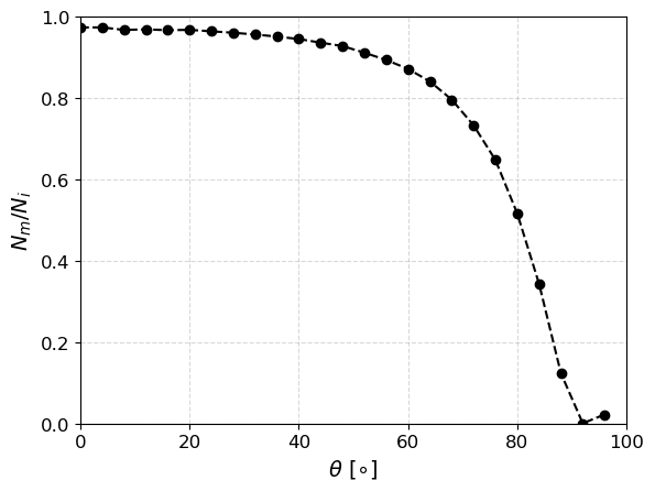
Number of simulated events: 10000000
Number of events that reached watched volume: 8532459
Working with a Response File
Once we have a response file, we can start by loading it directly. For example, the response file can be loaded as follows:
[3]:
instance.load_response("atm_response_33p5km.hdf5")
Below we show some more options for working with a response file.
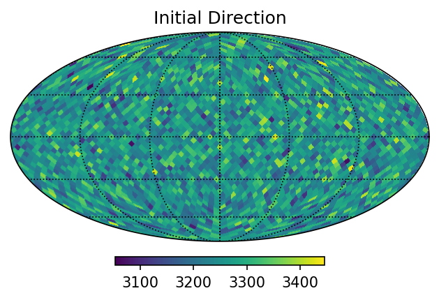
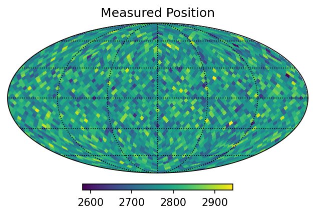
Make diagnostic plots
Note that numerous plots are made by default. We can turn off any of the plots if we want. See the API for more information.
[4]:
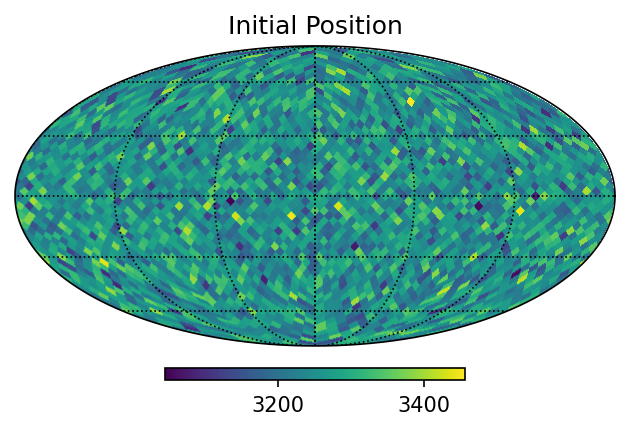
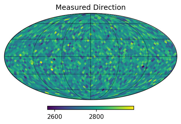
instance.make_scattering_plots(rsp_file="atm_response_33p5km.hdf5", ang_dist=[50,8000], pos_init=False, pos_meas=False, pos_proj=False)
/zfs/astrohe/ckarwin/My_Class_Library/COSI/cosi-atmosphere/cosi_atmosphere/response/ProcessSphericalSims.py:584: RuntimeWarning: invalid value encountered in sqrt
  rdisk = np.sqrt(self.radial_bins**2 - rsphere**2)
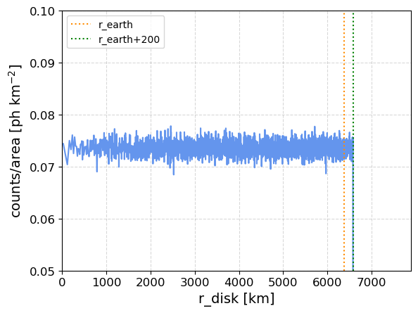
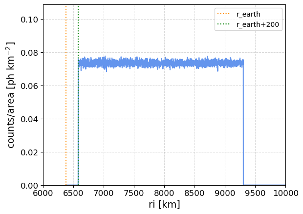
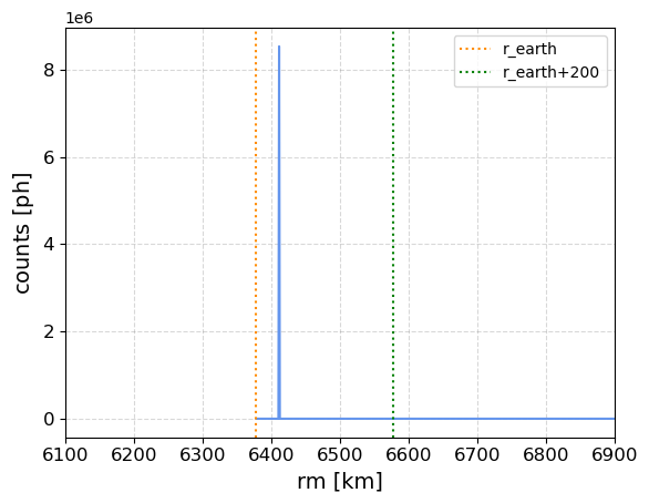
calculation of uniform flux through hemisphere:
radius of hemisphere [km]: 6411.600000000001
mean rate from surrounding sphere disk [ph/km^2]: 0.07356179254201645
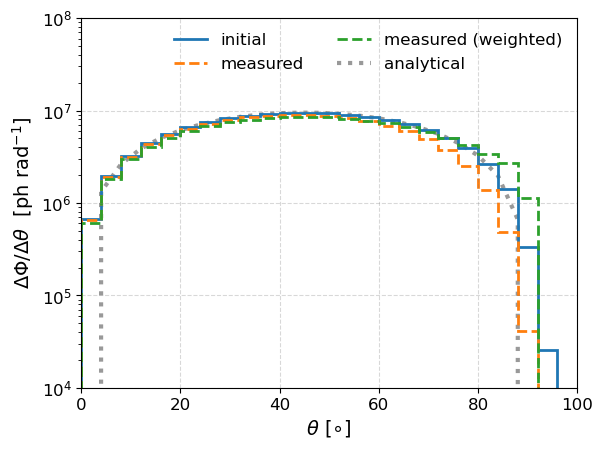
Using incident angle of 50 deg
Corresponding to angular bin 12
Using energy of 8000 keV
Corresponding to energy bin 15
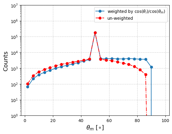
Initial energy distribution:
underflow bin: 0.0
overflow bin: 0.0
Measured energy distribution
underflow bin: 35.0
overflow bin: 0.0
Number of starting photons: 10000000.0
Number of measured photons: 8532424.0
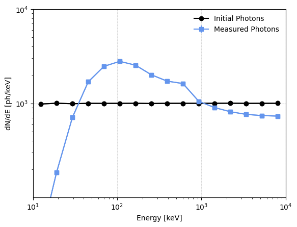
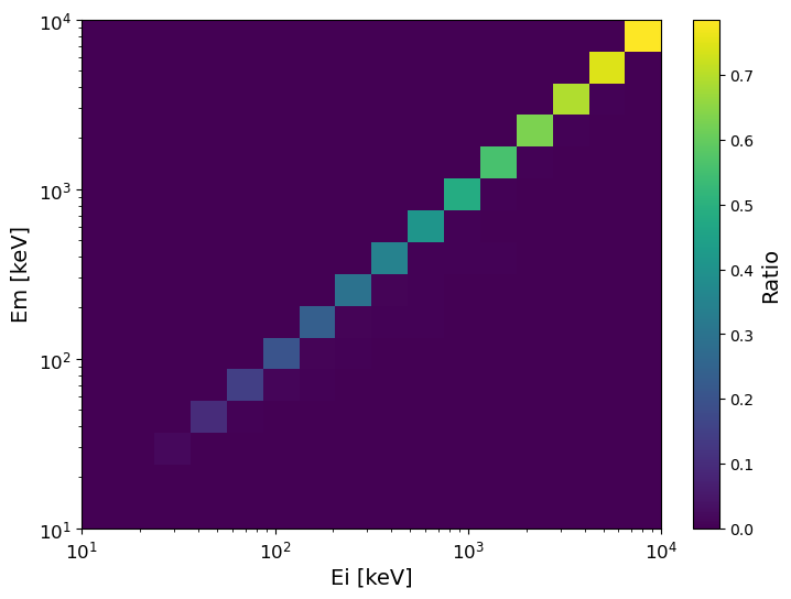
Make energy dispersion matrices
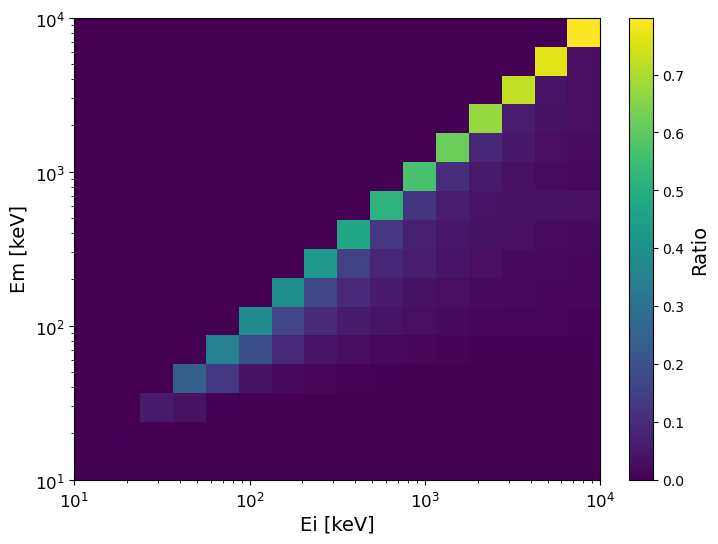
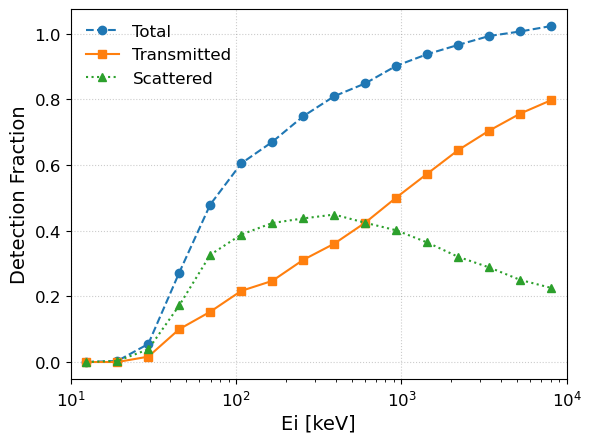
We’ll use an off-axis angle of 50 degrees. This will make energy dispersion matrices for both the transmitted and direct components, as well as the total. It will also make the detection fraction, which is equivalent to the transmission probability for the transmitted component.
[5]:
instance.get_total_edisp_matrix(50,rsp_file="atm_response_33p5km.hdf5")
Total number of photons in response normalization:
9531147.0

plotting transmitted edisp matrix...
/zfs/astrohe/Software/COSIMain_u2/lib/python3.9/site-packages/histpy/histogram.py:1301: RuntimeWarning: divide by zero encountered in divide
  self._contents = operation(self.full_contents, other)
/zfs/astrohe/Software/COSIMain_u2/lib/python3.9/site-packages/histpy/histogram.py:1301: RuntimeWarning: invalid value encountered in divide
  self._contents = operation(self.full_contents, other)
plotting scattered edisp matrix...
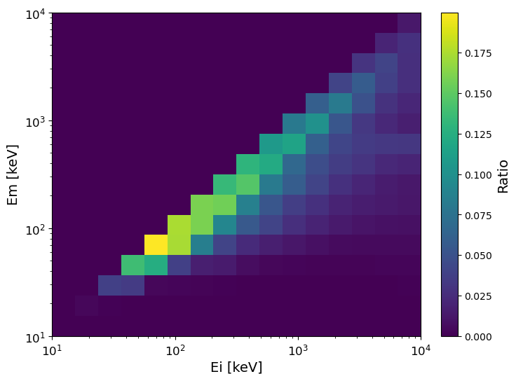
plotting total edisp matrix...
plotting transmission probability...
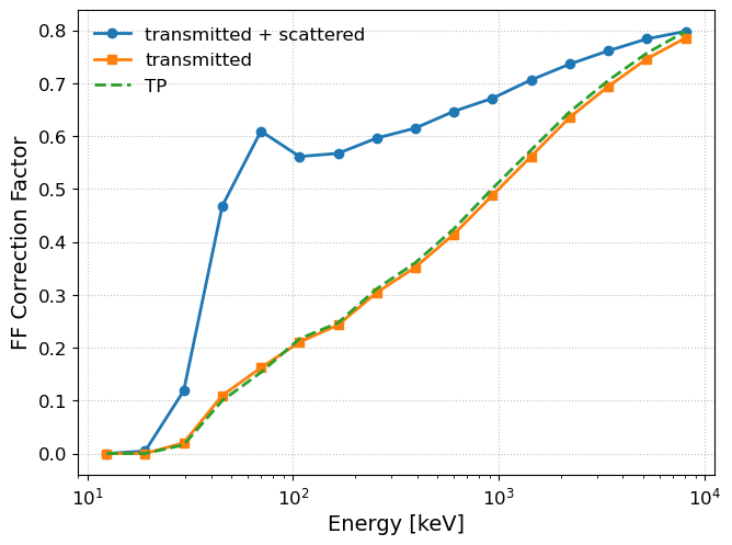
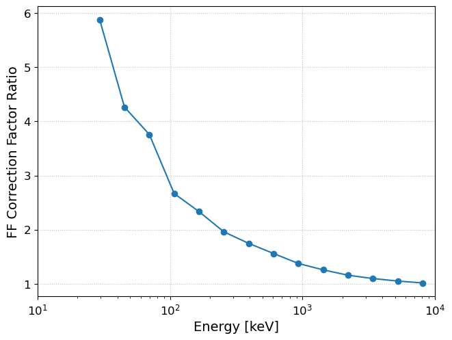
Calculate correction factors
After the energy dispersion matrices have been calcualted, we can calculate the correction factor and correction factor ratio. Let’s use a power law spectral model with an index of 2:
[6]:
model_flux=instance.PL_interp(2)
instance.ff_correction(model_flux,"output")
/zfs/astrohe/ckarwin/My_Class_Library/COSI/cosi-atmosphere/cosi_atmosphere/response/ProcessSims.py:846: RuntimeWarning: divide by zero encountered in divide
  c_ratio = c_total/c_beam