Simulating gamma-ray transport in the atmosphere using the rectangular mass model
This tutorial will demonstrate the basic functionality of the rectangular atmospheric mass model. For more details about the simulation and analysis pipeline, see Atmospheric Response for MeV Gamma Rays Observed with Balloon-Borne Detectors (Karwin+24).
Import the COSI atmosphere package
[1]:
from cosi_atmosphere.response.AtmosphericProfile import Atmosphere
from cosi_atmosphere.response.MassModels import MakeMassModels
from cosi_atmosphere.response.RunSims import Simulate
from cosi_atmosphere.response.ProcessSims import Process
import numpy as np
import os
This tutorial requires two files, which contain the photon data for a simulation using 1e6 photons. The files are hosted on wasabi, and they can be downloaded using the two cells below.
[ ]:
%%capture
# File size: ~ 109MB
os.system("AWS_ACCESS_KEY_ID=GBAL6XATQZNRV3GFH9Y4 AWS_SECRET_ACCESS_KEY=GToOczY5hGX3sketNO2fUwiq4DJoewzIgvTCHoOv aws s3api get-object  --bucket cosi-pipeline-public --key COSI-Atmosphere/Rectangular_Mass_Model_Tutorial/event_list_rectangular_geo_on_axis.dat --endpoint-url=https://s3.us-west-1.wasabisys.com event_list_rectangular_geo_on_axis.dat")
[ ]:
%%capture
# File size: ~ 115MB
os.system("AWS_ACCESS_KEY_ID=GBAL6XATQZNRV3GFH9Y4 AWS_SECRET_ACCESS_KEY=GToOczY5hGX3sketNO2fUwiq4DJoewzIgvTCHoOv aws s3api get-object  --bucket cosi-pipeline-public --key COSI-Atmosphere/Rectangular_Mass_Model_Tutorial/all_thrown_events_rectangular_geo_on_axis.dat --endpoint-url=https://s3.us-west-1.wasabisys.com all_thrown_events_rectangular_geo_on_axis.dat")
Make the Mass Model
The first step is to make an atmospheric model using the Atmosphere class. This provides an altitude density profile for the different species of the atmosphere. For the atmospheric model you need to specify the date, latitude and longitude, as well as the atmospheric spacing. Here we will use a spacing of 100 m.
[2]:
instance = Atmosphere()
date = np.array(['2016-06-13 12:00:00'], dtype="datetime64[h]")
lat = -5.66
lon = -107.38
alts = np.linspace(0, 200, 2001) # km; spacing is 0.1 km (100 m)
atm_model = instance.get_atm_profile("rep_atm_model.dat",date,lon,lat,alts)
Let’s take a look at the first 5 lines of the output file to see what it contains:
[3]:
%%capture
os.system("head -n 5 rep_atm_model.dat")
altitude[km]    mass_density[kg/m3]     N2[m-3] O2[m-3] O[m-3]  He[m-3] H[m-3]  Ar[m-3] N[m-3]  anomalous_oxygen[m-3]   NO[m-3] Temperature[k]
0.000000e+00    1.176653e+00    1.911429e+25    5.125639e+24    0.000000e+00    1.272904e+20    0.000000e+00    2.284374e+23    0.000000e+00    0.000000e+00    0.000000e+00    2.966827e+02
1.000000e-01    1.164742e+00    1.892081e+25    5.073756e+24    0.000000e+00    1.260020e+20    0.000000e+00    2.261251e+23    0.000000e+00    0.000000e+00    0.000000e+00    2.962918e+02
2.000000e-01    1.152961e+00    1.872944e+25    5.022437e+24    0.000000e+00    1.247275e+20    0.000000e+00    2.238379e+23    0.000000e+00    0.000000e+00    0.000000e+00    2.958947e+02
3.000000e-01    1.141304e+00    1.854006e+25    4.971656e+24    0.000000e+00    1.234664e+20    0.000000e+00    2.215747e+23    0.000000e+00    0.000000e+00    0.000000e+00    2.954918e+02
Next we need to make a mass model of the atmosphere. This is done with the MakeMassModels class, which takes as input the atmospheric model calculated in the previous step. Let’s first define an instance of the class and plot the atmospheric profile:
[4]:
instance = MakeMassModels("rep_atm_model.dat")
instance.plot_atmosphere()

The left axis in the above plot shows the number density of the different atmospheric elements. The right axis shows the total mass density of all elements.
Now let’s define our mass model. Two options are available for this: rectangular and spherical. The simulations use a watched volume to detect all passing photons, and so we need to pass the altitude to use. Here we will use a rectangular geometry with a watched volume at 33 km.
[5]:
instance.rectangular_model(33.5)
Using half-height [cm]: 5000.0
Watch index: 335
The output is written to atmosphere.geo. Let’s take a look at the first 40 lines:
[6]:
%%capture
os.system("head -n 40 atmosphere.geo")
# Atmosphere model

Name AtmoshpereModel

# Surrounding sphere:
SurroundingSphere 0.1 0 0 20000000.0 0.1

Volume World
World.Material Vacuum
World.Shape BOX 10240000000.000000 10240000000.000000 10240000000.000000
World.Visibility 1
World.Position 0 0 0
World.Mother 0

Include $(MEGALIB)/resource/examples/geomega/materials/Materials.geo

Material MaterialSlice_0_1
MaterialSlice_0_1.Density 0.001176653
MaterialSlice_0_1.ComponentByAtoms He 2
MaterialSlice_0_1.ComponentByAtoms N 784845
MaterialSlice_0_1.ComponentByAtoms O 210462
MaterialSlice_0_1.ComponentByAtoms Ar 4689

Volume VolumeSlice_0_1
VolumeSlice_0_1.Material MaterialSlice_0_1
VolumeSlice_0_1.Shape BOX 51200000.000000 51200000.000000 5000.0
VolumeSlice_0_1.Visibility  1
VolumeSlice_0_1.Position 0 0 5000.0
VolumeSlice_0_1.Mother World

Material MaterialSlice_1_2
MaterialSlice_1_2.Density 0.0011647419999999999
MaterialSlice_1_2.ComponentByAtoms He 2
MaterialSlice_1_2.ComponentByAtoms N 784845
MaterialSlice_1_2.ComponentByAtoms O 210462
MaterialSlice_1_2.ComponentByAtoms Ar 4689

Volume VolumeSlice_1_2
VolumeSlice_1_2.Material MaterialSlice_1_2
VolumeSlice_1_2.Shape BOX 51200000.000000 51200000.000000 5000.0
You can see that each volume slice is a large rectangular slab with a half-width of 5000 cm. The material of each volume slice corresponds to the atmospheric profile.
Now let’s take a look at the last 20 lines of the geometry file:
[7]:
%%capture
os.system("tail -n 20 atmosphere.geo")
MaterialSlice_1999_2000.Density 1.783777e-13
MaterialSlice_1999_2000.ComponentByAtoms H 81
MaterialSlice_1999_2000.ComponentByAtoms He 1311
MaterialSlice_1999_2000.ComponentByAtoms N 587675
MaterialSlice_1999_2000.ComponentByAtoms O 410776
MaterialSlice_1999_2000.ComponentByAtoms Ar 155

Volume VolumeSlice_1999_2000
VolumeSlice_1999_2000.Material MaterialSlice_1999_2000
VolumeSlice_1999_2000.Shape BOX 51200000.000000 51200000.000000 5000.0
VolumeSlice_1999_2000.Visibility  1
VolumeSlice_1999_2000.Position 0 0 19995000.0
VolumeSlice_1999_2000.Mother World

Volume TestVolume
TestVolume.Material MaterialSlice_335_336
TestVolume.Shape BOX 51200000.000000 51200000.000000 5000.0
TestVolume.Visibility 1
TestVolume.Position 0 0 0
TestVolume.Mother VolumeSlice_335_336
The last block here is our watched volume (called TestVolume). Here we are watching VolumeSlice_330_331, which corresponds to the rectangular slab at an altitude of 33 km. In principle, we can let the watched volume be whatever we want. For example, to use a sphere with a radius of 100 cm within the same volume slice, you would replace the shape with: TestVolume.Shape Sphere 0 100. This option is not yet hard coded, so if a different watched volume is needed, you will have to do it by hand for now.
Make the Source File
The other thing we need for the simulations is the source file. For the rectangular geometry we use a narrow beam, and an example file is provided: AtmospherePencilBeam.source. Let’s take a look:
[8]:
%%capture
os.system("cat AtmospherePencilBeam.source")
# An atmosphere simulation

Version         1
Geometry        atmosphere.geo

# Physics list
PhysicsListEM                        LivermorePol
PhysicsListEMActivateFluorescence    false

# Output formats
StoreCalibrated                      true
StoreSimulationInfo                  init-only
StoreSimulationInfoIonization        false
StoreSimulationInfoWatchedVolumes    TestVolume
StoreOnlyTriggeredEvents             false
DiscretizeHits                       true

DefaultRangeCut 100

Run SpaceSim
SpaceSim.FileName         AtmospherePencilBeam
SpaceSim.Triggers         100

# Attention: Concerning the lower energy band:
# The analysis is planned to be performed above 1 MeV.
# Therfore you set the lower energy limit for the simulation, well below this limit,
# to avoid problems due to energy resolution limitations

SpaceSim.Source Beam
Beam.ParticleType           1
Beam.Beam                   HomogeneousBeam 0 0 20000000   0 0 -1  1
Beam.Spectrum               Linear 10 10000
Beam.Flux                   1.0
For demonstration purposes we are only simulating 100 triggers. In practice, ~ 1 million - 5 million should provide sufficient statistics. We have a homogeneous narrow beam (r = 1cm) placed on axis at the top of the atmosphere (200 km), which throws photons straight down. The spectrum is linear between 10 - 10000 keV. The watched volume is placed at 33.5 km.
The inputs for HomogeneousBeam are: x y z nx ny nz r. We can place the beam off-axis by changing x, nx, and nz. For example, suppose we want to do 50 degrees off axis with a watched altitude of 33 km. We can determine what values we need to use by running the following:
[9]:
angle = 50.0 # degrees
altitude = 33.1 # km; be sure to account for slab thickness!
instance.get_cart_vectors(angle, altitude)
x [cm]: 19890367.460397366
nx [cm]: -0.766044443118978
nz [cm]: -0.6427876096865394
Replacing the corresponding inputs in the source file with these values will produce an off-axis source.
Run the Simulations
Once we have the mass model and the source file, we can run the simulations. Let’s define an instance of the Simulation class and make a short run.
[10]:
instance = Simulate()
instance.run_sim("AtmospherePencilBeam.source", seed=3000, verbosity=0)
**************************************************************************
*                                                                        *
*                Cosima - the cosmic simulator of MEGAlib                *
*                                                                        *
*             This program is part of MEGAlib version 3.99.02            *
*                (C) by Andreas Zoglauer and contributors                *
*                                                                        *
*                      Master reference for MEGAlib:                     *
*            A. Zoglauer et al., NewAR 50 (7-8), 629-632, 2006           *
*                                                                        *
*            For more information about MEGAlib please visit:            *
*                        http://megalibtoolkit.com                       *
*                                                                        *
**************************************************************************

              You are using a development version of MEGAlib

Using verbosity 0
Beam: Final flux: 1 ph/sec

*************************************************************
 Geant4 version Name: geant4-10-02-patch-03    (27-January-2017)
                      Copyright : Geant4 Collaboration
                      Reference : NIM A 506 (2003), 250-303
                            WWW : http://cern.ch/geant4
*************************************************************

Chosen physics:
Particles
G4EmLivermorePolarizedPhysics
G4RadioactiveDecay

Beam: Final flux: 1 ph/sec
Visualization Manager instantiating with verbosity "warnings (3)"...
Visualization Manager initialising...
Registering graphics systems...

You have successfully registered the following graphics systems.
Current available graphics systems are:
ASCIITree (ATree)
DAWNFILE (DAWNFILE)
G4HepRep (HepRepXML)
G4HepRepFile (HepRepFile)
RayTracer (RayTracer)
VRML1FILE (VRML1FILE)
VRML2FILE (VRML2FILE)
gMocrenFile (gMocrenFile)

Registering model factories...

You have successfully registered the following model factories.
Registered model factories:
  generic
  drawByCharge
  drawByParticleID
  drawByOriginVolume
  drawByAttribute

Registered filter factories:
  chargeFilter
  particleFilter
  originVolumeFilter
  attributeFilter

You have successfully registered the following user vis actions.
Run Duration User Vis Actions: none
End of Event User Vis Actions: none
End of Run User Vis Actions: none

Some /vis commands (optionally) take a string to specify colour.
Available colours:
  black, blue, brown, cyan, gray, green, grey, magenta, red, white, yellow


### ===  Deexcitation model UAtomDeexcitation is activated for 1 region:
          DefaultRegionForTheWorld

### === G4UAtomicDeexcitation::InitialiseForNewRun()
### ===  PIXE model for hadrons: Empirical
### ===  PIXE model for e+-:     Livermore

phot:   for  gamma    SubType= 12  BuildTable= 0
      LambdaPrime table from 200 keV to 10 TeV in 154 bins
      ===== EM models for the G4Region  DefaultRegionForTheWorld ======
LivermorePolarizedPhotoElectric :  Emin=        0 eV    Emax=        1 GeV   AngularGenSauterGavrilaPolarized  FluoActive
       PhotoElectric :  Emin=        1 GeV   Emax=       10 TeV   AngularGenSauterGavrila  FluoActive

compt:   for  gamma    SubType= 13  BuildTable= 1
      Lambda table from 100 eV  to 1 MeV, 20 bins per decade, spline: 1
      LambdaPrime table from 1 MeV to 10 TeV in 140 bins
      ===== EM models for the G4Region  DefaultRegionForTheWorld ======
LivermorePolarizedCompton :  Emin=        0 eV    Emax=        1 GeV  FluoActive
       Klein-Nishina :  Emin=        1 GeV   Emax=       10 TeV

conv:   for  gamma    SubType= 14  BuildTable= 1
      Lambda table from 1.022 MeV to 10 TeV, 20 bins per decade, spline: 1
      ===== EM models for the G4Region  DefaultRegionForTheWorld ======
LivermorePolarizedGammaConversion :  Emin=        0 eV    Emax=        1 GeV
        BetheHeitler :  Emin=        1 GeV   Emax=       80 GeV
     BetheHeitlerLPM :  Emin=       80 GeV   Emax=       10 TeV

Rayl:   for  gamma    SubType= 11  BuildTable= 1
      Lambda table from 100 eV  to 100 keV, 20 bins per decade, spline: 0
      LambdaPrime table from 100 keV to 10 TeV in 160 bins
      ===== EM models for the G4Region  DefaultRegionForTheWorld ======
LivermorePolarizedRayleigh :  Emin=        0 eV    Emax=        1 GeV
   LivermoreRayleigh :  Emin=        1 GeV   Emax=       10 TeV   CullenGenerator

msc:   for e-    SubType= 10
      RangeFactor= 0.04, stepLimitType: 3, latDisplacement: 1, skin= 1, geomFactor= 2.5
      ===== EM models for the G4Region  DefaultRegionForTheWorld ======
            UrbanMsc :  Emin=        0 eV    Emax=      100 MeV  Table with 120 bins Emin=    100 eV    Emax=    100 MeV
        WentzelVIUni :  Emin=      100 MeV   Emax=       10 TeV  Table with 100 bins Emin=    100 MeV   Emax=     10 TeV

CoulombScat:   for  e-, integral: 1     SubType= 1  BuildTable= 1
      Lambda table from 100 MeV to 10 TeV, 20 bins per decade, spline: 1
      180 < Theta(degree) < 180; pLimit(GeV^1)= 0.139531
      ===== EM models for the G4Region  DefaultRegionForTheWorld ======
  eCoulombScattering :  Emin=      100 MeV   Emax=       10 TeV

eIoni:   for  e-    SubType= 2
      dE/dx and range tables from 100 eV  to 10 TeV in 220 bins
      Lambda tables from threshold to 10 TeV, 20 bins per decade, spline: 1
      finalRange(mm)= 0.1, dRoverRange= 0.2, integral: 1, fluct: 1, linLossLimit= 0.01
      ===== EM models for the G4Region  DefaultRegionForTheWorld ======
       LowEnergyIoni :  Emin=        0 eV    Emax=      100 keV   deltaVI
        MollerBhabha :  Emin=      100 keV   Emax=       10 TeV   deltaVI

eBrem:   for  e-    SubType= 3
      dE/dx and range tables from 100 eV  to 10 TeV in 220 bins
      Lambda tables from threshold to 10 TeV, 20 bins per decade, spline: 1
      LPM flag: 1 for E > 1 GeV,  HighEnergyThreshold(GeV)= 10000
      ===== EM models for the G4Region  DefaultRegionForTheWorld ======
             eBremSB :  Emin=        0 eV    Emax=        1 GeV   DipBustGen
            eBremLPM :  Emin=        1 GeV   Emax=       10 TeV   DipBustGen

msc:   for e+    SubType= 10
      RangeFactor= 0.04, stepLimitType: 3, latDisplacement: 1, skin= 1, geomFactor= 2.5
      ===== EM models for the G4Region  DefaultRegionForTheWorld ======
            UrbanMsc :  Emin=        0 eV    Emax=      100 MeV  Table with 120 bins Emin=    100 eV    Emax=    100 MeV
        WentzelVIUni :  Emin=      100 MeV   Emax=       10 TeV  Table with 100 bins Emin=    100 MeV   Emax=     10 TeV

eIoni:   for  e+    SubType= 2
      dE/dx and range tables from 100 eV  to 10 TeV in 220 bins
      Lambda tables from threshold to 10 TeV, 20 bins per decade, spline: 1
      finalRange(mm)= 0.1, dRoverRange= 0.2, integral: 1, fluct: 1, linLossLimit= 0.01
      ===== EM models for the G4Region  DefaultRegionForTheWorld ======
        MollerBhabha :  Emin=        0 eV    Emax=       10 TeV   deltaVI

eBrem:   for  e+    SubType= 3
      dE/dx and range tables from 100 eV  to 10 TeV in 220 bins
      Lambda tables from threshold to 10 TeV, 20 bins per decade, spline: 1
      LPM flag: 1 for E > 1 GeV,  HighEnergyThreshold(GeV)= 10000
      ===== EM models for the G4Region  DefaultRegionForTheWorld ======
             eBremSB :  Emin=        0 eV    Emax=        1 GeV   DipBustGen
            eBremLPM :  Emin=        1 GeV   Emax=       10 TeV   DipBustGen

annihil:   for  e+, integral: 1     SubType= 5  BuildTable= 0
      ===== EM models for the G4Region  DefaultRegionForTheWorld ======
            eplus2gg :  Emin=        0 eV    Emax=       10 TeV

CoulombScat:   for  e+, integral: 1     SubType= 1  BuildTable= 1
      Lambda table from 100 MeV to 10 TeV, 20 bins per decade, spline: 1
      180 < Theta(degree) < 180; pLimit(GeV^1)= 0.139531
      ===== EM models for the G4Region  DefaultRegionForTheWorld ======
  eCoulombScattering :  Emin=      100 MeV   Emax=       10 TeV

msc:   for proton    SubType= 10
      RangeFactor= 0.2, step limit type: 0, lateralDisplacement: 0, polarAngleLimit(deg)= 180
      ===== EM models for the G4Region  DefaultRegionForTheWorld ======
        WentzelVIUni :  Emin=        0 eV    Emax=       10 TeV  Table with 220 bins Emin=    100 eV    Emax=     10 TeV

hIoni:   for  proton    SubType= 2
      dE/dx and range tables from 100 eV  to 10 TeV in 220 bins
      Lambda tables from threshold to 10 TeV, 20 bins per decade, spline: 1
      finalRange(mm)= 0.05, dRoverRange= 0.2, integral: 1, fluct: 1, linLossLimit= 0.01
      ===== EM models for the G4Region  DefaultRegionForTheWorld ======
               Bragg :  Emin=        0 eV    Emax=        2 MeV   deltaVI
          BetheBloch :  Emin=        2 MeV   Emax=       10 TeV   deltaVI

hBrems:   for  proton    SubType= 3
      dE/dx and range tables from 100 eV  to 10 TeV in 220 bins
      Lambda tables from threshold to 10 TeV, 20 bins per decade, spline: 1
      ===== EM models for the G4Region  DefaultRegionForTheWorld ======
               hBrem :  Emin=        0 eV    Emax=       10 TeV

hPairProd:   for  proton    SubType= 4
      dE/dx and range tables from 100 eV  to 10 TeV in 220 bins
      Lambda tables from threshold to 10 TeV, 20 bins per decade, spline: 1
      Sampling table 13x1001; from 7.50618 GeV to 10 TeV
      ===== EM models for the G4Region  DefaultRegionForTheWorld ======
           hPairProd :  Emin=        0 eV    Emax=       10 TeV

nuclearStopping:   for  proton    SubType= 8  BuildTable= 0
      ===== EM models for the G4Region  DefaultRegionForTheWorld ======
   ICRU49NucStopping :  Emin=        0 eV    Emax=        1 MeV

CoulombScat:   for  proton, integral: 1     SubType= 1  BuildTable= 1
      Lambda table from threshold  to 10 TeV, 20 bins per decade, spline: 1
      180 < Theta(degree) < 180; pLimit(GeV^1)= 0.139531
      ===== EM models for the G4Region  DefaultRegionForTheWorld ======
  eCoulombScattering :  Emin=        0 eV    Emax=       10 TeV

msc:   for GenericIon    SubType= 10
      RangeFactor= 0.2, stepLimitType: 0, latDisplacement: 0
      ===== EM models for the G4Region  DefaultRegionForTheWorld ======
            UrbanMsc :  Emin=        0 eV    Emax=       10 TeV

ionIoni:   for  GenericIon    SubType= 2
      dE/dx and range tables from 100 eV  to 10 TeV in 220 bins
      Lambda tables from threshold to 10 TeV, 20 bins per decade, spline: 1
      finalRange(mm)= 0.001, dRoverRange= 0.1, integral: 1, fluct: 1, linLossLimit= 0.02
      ===== EM models for the G4Region  DefaultRegionForTheWorld ======
         ParamICRU73 :  Emin=        0 eV    Emax=       10 TeV   deltaVI

nuclearStopping:   for  GenericIon    SubType= 8  BuildTable= 0
      ===== EM models for the G4Region  DefaultRegionForTheWorld ======
   ICRU49NucStopping :  Emin=        0 eV    Emax=        1 MeV

### ===  Deexcitation model UAtomDeexcitation is activated for 1 region:
          DefaultRegionForTheWorld

### === G4UAtomicDeexcitation::InitialiseForNewRun()
### ===  PIXE model for hadrons: Empirical
### ===  PIXE model for e+-:     Livermore

msc:   for alpha    SubType= 10
      RangeFactor= 0.2, stepLimitType: 0, latDisplacement: 0
      ===== EM models for the G4Region  DefaultRegionForTheWorld ======
            UrbanMsc :  Emin=        0 eV    Emax=       10 TeV  Table with 220 bins Emin=    100 eV    Emax=     10 TeV

ionIoni:   for  alpha    SubType= 2
      dE/dx and range tables from 100 eV  to 10 TeV in 220 bins
      Lambda tables from threshold to 10 TeV, 20 bins per decade, spline: 1
      finalRange(mm)= 0.01, dRoverRange= 0.1, integral: 1, fluct: 1, linLossLimit= 0.02
      ===== EM models for the G4Region  DefaultRegionForTheWorld ======
            BraggIon :  Emin=        0 eV    Emax=   7.9452 MeV   deltaVI
          BetheBloch :  Emin=   7.9452 MeV   Emax=       10 TeV   deltaVI

nuclearStopping:   for  alpha    SubType= 8  BuildTable= 0
      ===== EM models for the G4Region  DefaultRegionForTheWorld ======
   ICRU49NucStopping :  Emin=        0 eV    Emax=        1 MeV

msc:   for anti_proton    SubType= 10
      RangeFactor= 0.2, step limit type: 0, lateralDisplacement: 0, polarAngleLimit(deg)= 180
      ===== EM models for the G4Region  DefaultRegionForTheWorld ======
        WentzelVIUni :  Emin=        0 eV    Emax=       10 TeV  Table with 220 bins Emin=    100 eV    Emax=     10 TeV

hIoni:   for  anti_proton    SubType= 2
      dE/dx and range tables from 100 eV  to 10 TeV in 220 bins
      Lambda tables from threshold to 10 TeV, 20 bins per decade, spline: 1
      finalRange(mm)= 0.05, dRoverRange= 0.2, integral: 1, fluct: 1, linLossLimit= 0.01
      ===== EM models for the G4Region  DefaultRegionForTheWorld ======
            ICRU73QO :  Emin=        0 eV    Emax=        2 MeV   deltaVI
          BetheBloch :  Emin=        2 MeV   Emax=       10 TeV   deltaVI

hBrems:   for  anti_proton    SubType= 3
      dE/dx and range tables from 100 eV  to 10 TeV in 220 bins
      Lambda tables from threshold to 10 TeV, 20 bins per decade, spline: 1
      ===== EM models for the G4Region  DefaultRegionForTheWorld ======
               hBrem :  Emin=        0 eV    Emax=       10 TeV

hPairProd:   for  anti_proton    SubType= 4
      dE/dx and range tables from 100 eV  to 10 TeV in 220 bins
      Lambda tables from threshold to 10 TeV, 20 bins per decade, spline: 1
      Sampling table 13x1001; from 7.50618 GeV to 10 TeV
      ===== EM models for the G4Region  DefaultRegionForTheWorld ======
           hPairProd :  Emin=        0 eV    Emax=       10 TeV

nuclearStopping:   for  anti_proton    SubType= 8  BuildTable= 0
      ===== EM models for the G4Region  DefaultRegionForTheWorld ======
   ICRU49NucStopping :  Emin=        0 eV    Emax=        1 MeV

CoulombScat:   for  anti_proton, integral: 1     SubType= 1  BuildTable= 1
      Lambda table from threshold  to 10 TeV, 20 bins per decade, spline: 1
      180 < Theta(degree) < 180; pLimit(GeV^1)= 0.139531
      ===== EM models for the G4Region  DefaultRegionForTheWorld ======
  eCoulombScattering :  Emin=        0 eV    Emax=       10 TeV

msc:   for kaon+    SubType= 10
      RangeFactor= 0.2, step limit type: 0, lateralDisplacement: 0, polarAngleLimit(deg)= 180
      ===== EM models for the G4Region  DefaultRegionForTheWorld ======
        WentzelVIUni :  Emin=        0 eV    Emax=       10 TeV  Table with 220 bins Emin=    100 eV    Emax=     10 TeV

hIoni:   for  kaon+    SubType= 2
      dE/dx and range tables from 100 eV  to 10 TeV in 220 bins
      Lambda tables from threshold to 10 TeV, 20 bins per decade, spline: 1
      finalRange(mm)= 0.05, dRoverRange= 0.2, integral: 1, fluct: 1, linLossLimit= 0.01
      ===== EM models for the G4Region  DefaultRegionForTheWorld ======
               Bragg :  Emin=        0 eV    Emax=  1.05231 MeV   deltaVI
          BetheBloch :  Emin=  1.05231 MeV   Emax=       10 TeV   deltaVI

hBrems:   for  kaon+    SubType= 3
      dE/dx and range tables from 100 eV  to 10 TeV in 220 bins
      Lambda tables from threshold to 10 TeV, 20 bins per decade, spline: 1
      ===== EM models for the G4Region  DefaultRegionForTheWorld ======
               hBrem :  Emin=        0 eV    Emax=       10 TeV

hPairProd:   for  kaon+    SubType= 4
      dE/dx and range tables from 100 eV  to 10 TeV in 220 bins
      Lambda tables from threshold to 10 TeV, 20 bins per decade, spline: 1
      Sampling table 14x1001; from 3.94942 GeV to 10 TeV
      ===== EM models for the G4Region  DefaultRegionForTheWorld ======
           hPairProd :  Emin=        0 eV    Emax=       10 TeV

CoulombScat:   for  kaon+, integral: 1     SubType= 1  BuildTable= 1
      Lambda table from threshold  to 10 TeV, 20 bins per decade, spline: 1
      180 < Theta(degree) < 180; pLimit(GeV^1)= 0.139531
      ===== EM models for the G4Region  DefaultRegionForTheWorld ======
  eCoulombScattering :  Emin=        0 eV    Emax=       10 TeV

msc:   for kaon-    SubType= 10
      RangeFactor= 0.2, step limit type: 0, lateralDisplacement: 0, polarAngleLimit(deg)= 180
      ===== EM models for the G4Region  DefaultRegionForTheWorld ======
        WentzelVIUni :  Emin=        0 eV    Emax=       10 TeV  Table with 220 bins Emin=    100 eV    Emax=     10 TeV

hIoni:   for  kaon-    SubType= 2
      dE/dx and range tables from 100 eV  to 10 TeV in 220 bins
      Lambda tables from threshold to 10 TeV, 20 bins per decade, spline: 1
      finalRange(mm)= 0.05, dRoverRange= 0.2, integral: 1, fluct: 1, linLossLimit= 0.01
      ===== EM models for the G4Region  DefaultRegionForTheWorld ======
            ICRU73QO :  Emin=        0 eV    Emax=  1.05231 MeV   deltaVI
          BetheBloch :  Emin=  1.05231 MeV   Emax=       10 TeV   deltaVI

hBrems:   for  kaon-    SubType= 3
      dE/dx and range tables from 100 eV  to 10 TeV in 220 bins
      Lambda tables from threshold to 10 TeV, 20 bins per decade, spline: 1
      ===== EM models for the G4Region  DefaultRegionForTheWorld ======
               hBrem :  Emin=        0 eV    Emax=       10 TeV

hPairProd:   for  kaon-    SubType= 4
      dE/dx and range tables from 100 eV  to 10 TeV in 220 bins
      Lambda tables from threshold to 10 TeV, 20 bins per decade, spline: 1
      Sampling table 14x1001; from 3.94942 GeV to 10 TeV
      ===== EM models for the G4Region  DefaultRegionForTheWorld ======
           hPairProd :  Emin=        0 eV    Emax=       10 TeV

CoulombScat:   for  kaon-, integral: 1     SubType= 1  BuildTable= 1
      Lambda table from threshold  to 10 TeV, 20 bins per decade, spline: 1
      180 < Theta(degree) < 180; pLimit(GeV^1)= 0.139531
      ===== EM models for the G4Region  DefaultRegionForTheWorld ======
  eCoulombScattering :  Emin=        0 eV    Emax=       10 TeV

msc:   for mu+    SubType= 10
      RangeFactor= 0.2, step limit type: 0, lateralDisplacement: 0, polarAngleLimit(deg)= 180
      ===== EM models for the G4Region  DefaultRegionForTheWorld ======
        WentzelVIUni :  Emin=        0 eV    Emax=       10 TeV  Table with 220 bins Emin=    100 eV    Emax=     10 TeV

muIoni:   for  mu+    SubType= 2
      dE/dx and range tables from 100 eV  to 10 TeV in 220 bins
      Lambda tables from threshold to 10 TeV, 20 bins per decade, spline: 1
      finalRange(mm)= 0.05, dRoverRange= 0.2, integral: 1, fluct: 1, linLossLimit= 0.01
      ===== EM models for the G4Region  DefaultRegionForTheWorld ======
               Bragg :  Emin=        0 eV    Emax=      200 keV   deltaVI
          BetheBloch :  Emin=      200 keV   Emax=        1 GeV   deltaVI
        MuBetheBloch :  Emin=        1 GeV   Emax=       10 TeV

muBrems:   for  mu+    SubType= 3
      dE/dx and range tables from 100 eV  to 10 TeV in 220 bins
      Lambda tables from threshold to 10 TeV, 20 bins per decade, spline: 1
      ===== EM models for the G4Region  DefaultRegionForTheWorld ======
              MuBrem :  Emin=        0 eV    Emax=       10 TeV

muPairProd:   for  mu+    SubType= 4
      dE/dx and range tables from 100 eV  to 10 TeV in 220 bins
      Lambda tables from threshold to 10 TeV, 20 bins per decade, spline: 1
      Sampling table 17x1001; from 1 GeV to 10 TeV
      ===== EM models for the G4Region  DefaultRegionForTheWorld ======
          muPairProd :  Emin=        0 eV    Emax=       10 TeV

CoulombScat:   for  mu+, integral: 1     SubType= 1  BuildTable= 1
      Lambda table from threshold  to 10 TeV, 20 bins per decade, spline: 1
      180 < Theta(degree) < 180; pLimit(GeV^1)= 0.139531
      ===== EM models for the G4Region  DefaultRegionForTheWorld ======
  eCoulombScattering :  Emin=        0 eV    Emax=       10 TeV

msc:   for mu-    SubType= 10
      RangeFactor= 0.2, step limit type: 0, lateralDisplacement: 0, polarAngleLimit(deg)= 180
      ===== EM models for the G4Region  DefaultRegionForTheWorld ======
        WentzelVIUni :  Emin=        0 eV    Emax=       10 TeV  Table with 220 bins Emin=    100 eV    Emax=     10 TeV

muIoni:   for  mu-    SubType= 2
      dE/dx and range tables from 100 eV  to 10 TeV in 220 bins
      Lambda tables from threshold to 10 TeV, 20 bins per decade, spline: 1
      finalRange(mm)= 0.05, dRoverRange= 0.2, integral: 1, fluct: 1, linLossLimit= 0.01
      ===== EM models for the G4Region  DefaultRegionForTheWorld ======
            ICRU73QO :  Emin=        0 eV    Emax=      200 keV   deltaVI
          BetheBloch :  Emin=      200 keV   Emax=        1 GeV   deltaVI
        MuBetheBloch :  Emin=        1 GeV   Emax=       10 TeV

muBrems:   for  mu-    SubType= 3
      dE/dx and range tables from 100 eV  to 10 TeV in 220 bins
      Lambda tables from threshold to 10 TeV, 20 bins per decade, spline: 1
      ===== EM models for the G4Region  DefaultRegionForTheWorld ======
              MuBrem :  Emin=        0 eV    Emax=       10 TeV

muPairProd:   for  mu-    SubType= 4
      dE/dx and range tables from 100 eV  to 10 TeV in 220 bins
      Lambda tables from threshold to 10 TeV, 20 bins per decade, spline: 1
      Sampling table 17x1001; from 1 GeV to 10 TeV
      ===== EM models for the G4Region  DefaultRegionForTheWorld ======
          muPairProd :  Emin=        0 eV    Emax=       10 TeV

CoulombScat:   for  mu-, integral: 1     SubType= 1  BuildTable= 1
      Lambda table from threshold  to 10 TeV, 20 bins per decade, spline: 1
      180 < Theta(degree) < 180; pLimit(GeV^1)= 0.139531
      ===== EM models for the G4Region  DefaultRegionForTheWorld ======
  eCoulombScattering :  Emin=        0 eV    Emax=       10 TeV

msc:   for pi+    SubType= 10
      RangeFactor= 0.2, step limit type: 0, lateralDisplacement: 0, polarAngleLimit(deg)= 180
      ===== EM models for the G4Region  DefaultRegionForTheWorld ======
        WentzelVIUni :  Emin=        0 eV    Emax=       10 TeV  Table with 220 bins Emin=    100 eV    Emax=     10 TeV

hIoni:   for  pi+    SubType= 2
      dE/dx and range tables from 100 eV  to 10 TeV in 220 bins
      Lambda tables from threshold to 10 TeV, 20 bins per decade, spline: 1
      finalRange(mm)= 0.05, dRoverRange= 0.2, integral: 1, fluct: 1, linLossLimit= 0.01
      ===== EM models for the G4Region  DefaultRegionForTheWorld ======
               Bragg :  Emin=        0 eV    Emax=  297.505 keV   deltaVI
          BetheBloch :  Emin=  297.505 keV   Emax=       10 TeV   deltaVI

hBrems:   for  pi+    SubType= 3
      dE/dx and range tables from 100 eV  to 10 TeV in 220 bins
      Lambda tables from threshold to 10 TeV, 20 bins per decade, spline: 1
      ===== EM models for the G4Region  DefaultRegionForTheWorld ======
               hBrem :  Emin=        0 eV    Emax=       10 TeV

hPairProd:   for  pi+    SubType= 4
      dE/dx and range tables from 100 eV  to 10 TeV in 220 bins
      Lambda tables from threshold to 10 TeV, 20 bins per decade, spline: 1
      Sampling table 16x1001; from 1.11656 GeV to 10 TeV
      ===== EM models for the G4Region  DefaultRegionForTheWorld ======
           hPairProd :  Emin=        0 eV    Emax=       10 TeV

CoulombScat:   for  pi+, integral: 1     SubType= 1  BuildTable= 1
      Lambda table from threshold  to 10 TeV, 20 bins per decade, spline: 1
      180 < Theta(degree) < 180; pLimit(GeV^1)= 0.139531
      ===== EM models for the G4Region  DefaultRegionForTheWorld ======
  eCoulombScattering :  Emin=        0 eV    Emax=       10 TeV

msc:   for pi-    SubType= 10
      RangeFactor= 0.2, step limit type: 0, lateralDisplacement: 0, polarAngleLimit(deg)= 180
      ===== EM models for the G4Region  DefaultRegionForTheWorld ======
        WentzelVIUni :  Emin=        0 eV    Emax=       10 TeV  Table with 220 bins Emin=    100 eV    Emax=     10 TeV

hIoni:   for  pi-    SubType= 2
      dE/dx and range tables from 100 eV  to 10 TeV in 220 bins
      Lambda tables from threshold to 10 TeV, 20 bins per decade, spline: 1
      finalRange(mm)= 0.05, dRoverRange= 0.2, integral: 1, fluct: 1, linLossLimit= 0.01
      ===== EM models for the G4Region  DefaultRegionForTheWorld ======
            ICRU73QO :  Emin=        0 eV    Emax=  297.505 keV   deltaVI
          BetheBloch :  Emin=  297.505 keV   Emax=       10 TeV   deltaVI

hBrems:   for  pi-    SubType= 3
      dE/dx and range tables from 100 eV  to 10 TeV in 220 bins
      Lambda tables from threshold to 10 TeV, 20 bins per decade, spline: 1
      ===== EM models for the G4Region  DefaultRegionForTheWorld ======
               hBrem :  Emin=        0 eV    Emax=       10 TeV

hPairProd:   for  pi-    SubType= 4
      dE/dx and range tables from 100 eV  to 10 TeV in 220 bins
      Lambda tables from threshold to 10 TeV, 20 bins per decade, spline: 1
      Sampling table 16x1001; from 1.11656 GeV to 10 TeV
      ===== EM models for the G4Region  DefaultRegionForTheWorld ======
           hPairProd :  Emin=        0 eV    Emax=       10 TeV

CoulombScat:   for  pi-, integral: 1     SubType= 1  BuildTable= 1
      Lambda table from threshold  to 10 TeV, 20 bins per decade, spline: 1
      180 < Theta(degree) < 180; pLimit(GeV^1)= 0.139531
      ===== EM models for the G4Region  DefaultRegionForTheWorld ======
  eCoulombScattering :  Emin=        0 eV    Emax=       10 TeV


Summary for run SpaceSim

Total number of generated particles:     100
  Source Beam:                           100

Total CPU time spent in run:             16.77 sec
Time spent per event:                    0.1677 sec

Observation time:                        113.839 sec

Graphics systems deleted.
Visualization Manager deleting...
Process the simulations
The above command is a python wrapper for cosima, and it will produce the .sim file. Now let’s parse the sim file. This will produce two .dat files: one with information for all thrown photons and another with information for all detected photons.
[11]:
instance.parse_sim_file("AtmospherePencilBeam.inc1.id1.sim")
Let’s take a look at the output format:
[12]:
%%capture
os.system("head -n 5 all_thrown_events.dat")
id      ei[keV] xi[cm]  yi[cm]  zi[cm]  xdi[cm] ydi[cm] zdi[cm]
1       6.041339000e+03 7.339900000e-01 1.017700000e-01 2.000000000e+07 0.000000000e+00 0.000000000e+00 -1.000000000e+00
2       7.831685000e+03 6.970800000e-01 -4.249200000e-01        2.000000000e+07 0.000000000e+00 0.000000000e+00 -1.000000000e+00
3       3.470339000e+03 -1.828400000e-01        -2.275600000e-01        2.000000000e+07 0.000000000e+00 0.000000000e+00 -1.000000000e+00
4       6.729603000e+03 3.257600000e-01 7.572800000e-01 2.000000000e+07 0.000000000e+00 0.000000000e+00 -1.000000000e+00
[13]:
%%capture
os.system("head -n 5 event_list.dat")
id      em[keV] xm[cm]  ym[cm]  zm[cm]  xdm[cm] ydm[cm] zdm[cm]
1       6.041339000e+03 7.339900000e-01 1.017700000e-01 3.360000000e+06 0.000000000e+00 0.000000000e+00 -1.000000000e+00
2       7.831685000e+03 6.970800000e-01 -4.249200000e-01        3.360000000e+06 0.000000000e+00 0.000000000e+00 -1.000000000e+00
3       3.470339000e+03 -1.828400000e-01        -2.275600000e-01        3.360000000e+06 0.000000000e+00 0.000000000e+00 -1.000000000e+00
4       6.729603000e+03 3.257600000e-01 7.572800000e-01 3.360000000e+06 0.000000000e+00 0.000000000e+00 -1.000000000e+00
Note that the first file has all the initial information, and the second file has all the measured information.
Make response file
Now we can process the simulations using the Process class. When defining an instance of the Process class we need to specify off-axis angle of the source. For this example, we will use files downloaded at the beginning of the tutorial, which are for the same setup, but with 1 million simulated photons. These files can be specified when we initiate an instance of the class. Let’s bin the data and make the response file:
[14]:
instance = Process(0, all_events_file="all_thrown_events_rectangular_geo_on_axis.dat" , measured_events_file="event_list_rectangular_geo_on_axis.dat")
instance.bin_sim(rsp_name="atm_response.h5")
Now lets make some diagnostic plots:
[18]:
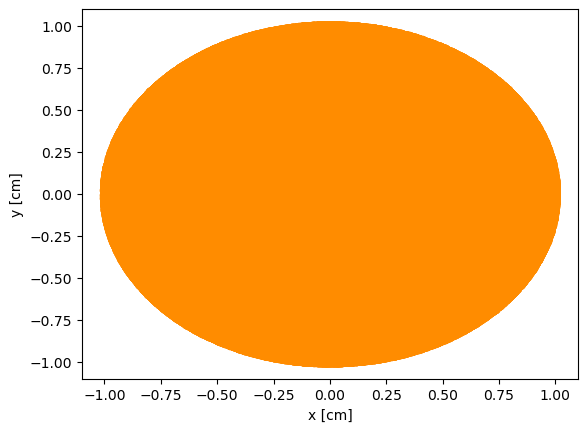
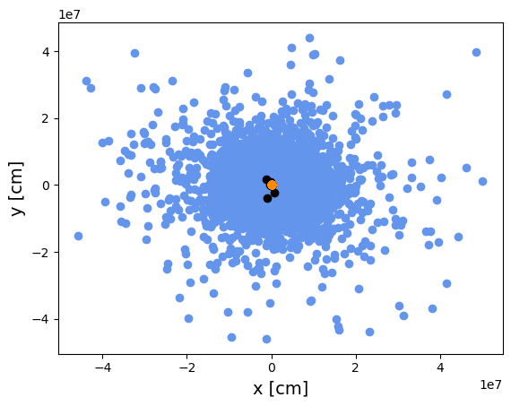
instance.make_scattering_plots(theta_prime_em = False, rad_em = False, rad_ei = False)
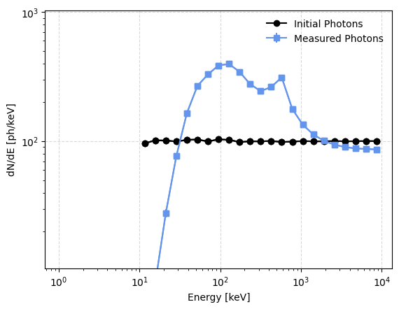
Number of starting photons: 1000000.0
Number of measured photons: 1065266.0095752797
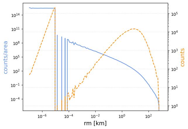
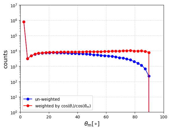
Summary of output plots: (1) x y positions of starting photons (2) x y positions of measured photons: blue = scatterd, black = un-scattered (3) spectrum of initial and measured photons (4) distribution of counts versus the radius from the center of the beam (5) distribution of counts versus the photon’s incident angle
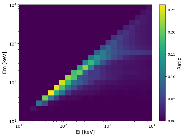
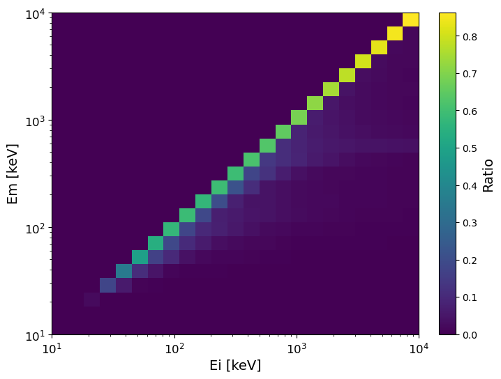
Make energy dispersion matrices and correction factors
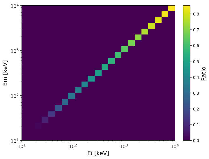
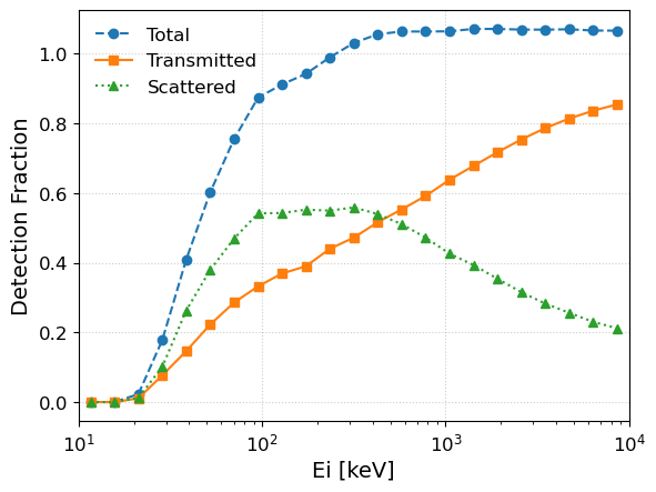
Now let’s get the atmospheric response. The first three outputs will show the energy dispersion matrices for the transmitted component, the scattered component, and the total (which is the sum of the transmitted and scattered components). The last output will show the detection fraction for all three components, which is the projection of the energy dispersion matrices onto the initial energy axis.
[16]:
instance.get_total_edisp_matrix()
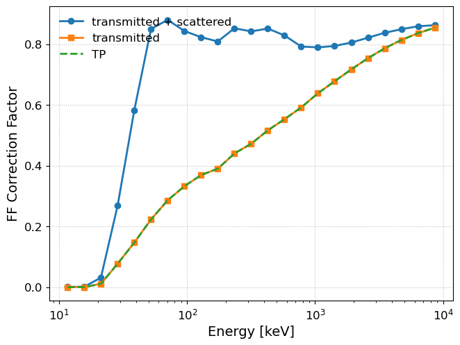
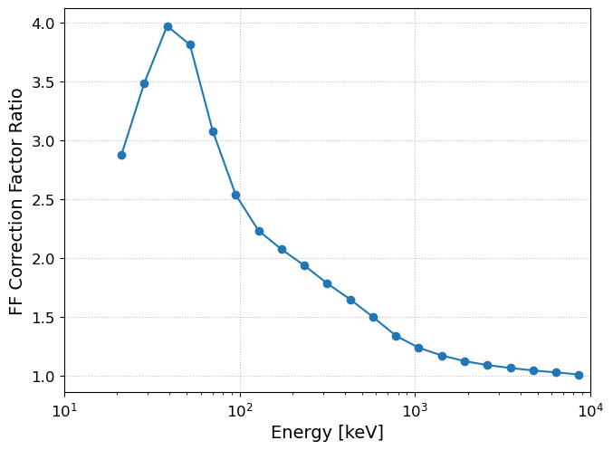
Finally, let’s get the correction factor and correction factor ratio (also defined in Karwin+23). We’ll use a power law spectral model with index 2.
[17]:
model_flux=instance.PL_interp(2)
instance.ff_correction(model_flux,"new_sims")
/zfs/astrohe/ckarwin/My_Class_Library/COSI/cosi-atmosphere/cosi_atmosphere/response/ProcessSims.py:867: RuntimeWarning: divide by zero encountered in divide
  c_ratio = c_total/c_beam